
Reinforcement learning or RL is a class of methods for solving various kinds of sequential decision making tasks. In such tasks, we want to design an agent that interacts with an external environment . The agent maintains an internal state \(z_t\), which it passes to its policy \(π\) to choose an action \(a_t = π(z_t)\). The environment responds by sending back an observation \(o_{t+1}\), which the agent uses to update its internal state using the state-update function \(z_{t+1} = SU (z_t, a_t, o_{t+1})\). See Figure 1.1 for an illustration.
強化学習またはRLは、さまざまな種類の逐次的な意思決定タスクを解決するための手法の一種です。このようなタスクでは、外部の環境と相互作用するエージェントを設計します。エージェントは内部状態 \(z_t\) を維持し、それをポリシー \(π\) に渡してアクション \(a_t = π(z_t)\) を選択します。環境は観測値 \(o_{t+1}\) を返して応答し、エージェントは状態更新関数 \(z_{t+1} = SU (z_t, a_t, o_{t+1})\) を使用して内部状態を更新します。図1.1に説明を示します。
Figure 1.1: A small agent interacting with a big external world. The observation \(o_t\) (which, for notational simplicity,
includes the previous action \(a_t\)) is used to update the internal agent state \(z_t\), which is passed to the policy \(π\) which
picks the next action \(a_{t+1}\) based on the agent's goal \(g_t\). Rewards are computed internally by the agent, by comparing \(z_t\)
with its internal goal \(g_t\). The observations, actions and rewards are stored in a replay buffer, which can be used to
learn the policy, a value function (not shown), and optionally an internal world model (for use in model-based RL, see
Chapter 4).
図1.1: 小さなエージェントが大きな外部世界と相互作用する様子。観測値 \(o_t\) (表記を簡略化するため、前の行動 \(a_t\) を含む) はエージェントの内部状態 zt を更新するために使用され、これは方策 \(π\) に渡され、方策 \(π\) はエージェントの目標 \(g_t\) に基づいて次の行動 \(a_{t+1}\) を選択する。報酬はエージェント内部で、\(z_t\) と内部目標 gt を比較することによって計算される。観測値、行動、報酬はリプレイバッファに保存され、方策、価値関数 (図示せず)、およびオプションで内部世界モデル (モデルベース強化学習で使用する場合は、第4章を参照) を学習するために使用できる。
To simplify things, we often assume that the environment is also a Markovian process, which has internal world state \(w_t\), from which the observations \(o_t\) are derived. (This is called a POMDP — see Section 1.2.1 ). We often simplify things even more by assuming that the observation \(o_t\) reveals the hidden environment state; in this case, we denote the internal agent state and external environment state by the same letter, namely \(s_t = o_t = w_t = z_t\). (This is called an MDP — see Section 1.2.2). We discuss these assumptions in more detail in Section 1.1.3.
物事を単純化するために、環境もマルコフ過程であり、内部世界状態 \(w_t\) を持ち、そこから観測 \(o_t\) が導出されると仮定することがよくあります。(これは POMDP と呼ばれます。セクション 1.2.1 を参照してください)。観測 \(o_t\) によって隠れた環境状態が明らかになると仮定することで、物事をさらに単純化することがよくあります。この場合、エージェントの内部状態と外部環境の状態を同じ文字で表し、\(s_t = o_t = w_t = z_t\) とします。(これは MDP と呼ばれます。セクション 1.2.2 を参照してください)。これらの仮定については、セクション 1.1.3 で詳しく説明します。
RL is more complicated than supervised learning (e.g., training a classifier) or self-supervised learning (e.g., training a language model), because this framework is very general: there are many assumptions we can make about the environment and its observations ot, and many choices we can make about the form the agent's internal state \(z_t\) and policy \(π\), as well the ways to update these objects as we see more data. We will study many different combinations in the rest of this document. The right choice ultimately depends on which real-world application you are interested in solving. 1
強化学習は、教師あり学習(例:分類器の学習)や自己教師あり学習(例:言語モデルの学習)よりも複雑です。これは、このフレームワークが非常に汎用的であるためです。環境とその観測値 ot について多くの仮定を置けますし、エージェントの内部状態 \(z_t\) と方策 \(π\) の形式についても多くの選択肢があり、さらにデータが増えていくにつれてこれらのオブジェクトを更新する方法も異なります。このドキュメントの残りの部分では、様々な組み合わせについて見ていきます。最終的に、適切な選択は、どのような現実世界のアプリケーションを解決したいかによって決まります。1
1
For a list of real-world applications of RL, see e.g.,
https://bit.ly/42V7dIJ from Csaba szepesvari (2024), https://bit. ly/3EMMYCW from Vitaly Kurin (2022), and https://github.com/montrealrobotics/DeepRLInTheWorld, which seems to be kept up to date.
RL の実際のアプリケーションのリストについては、例えば、Csaba szepesvari (2024) の https://bit.ly/42V7dIJ、Vitaly Kurin (2022) の https://bit.ly/3EMMYCW、および最新の状態に保たれていると思われる https://github.com/montrealrobotics/DeepRLInTheWorld を参照してください。
The goal of the agent is to choose a policy \(π\) so as to maximize the sum of expected rewards:
エージェントの目標は、期待報酬の合計を最大化するようにポリシー \(π\) を選択することです。
\[
V_π(s_0) = \mathbb{E}_{p(a_0,s_1,a_1,...,a_T ,s_T |s_0,π)}
\Bigg[\sum_{t=0}^T R(s_t, a_t)|s_0\Bigg] \tag{1.1}
\]
where \(s_0\) is the agent's initial state, \(R(s_t, a_t)\) is the reward function that the agent uses to measure the value of performing an action in a given state, \(V_π(s_0)\) is the value function for policy \(π\) evaluated at \(s_0\), and the expectation is wrt
ここで、\(s_0\)はエージェントの初期状態、\(R(s_t, a_t)\)はエージェントが特定の状態で行動を実行することの価値を測定するために使用する報酬関数、\(V_π(s_0)\)は\(s_0\)で評価されたポリシー\(π\)の価値関数であり、期待値はwrtである。
\[
\begin{align}
p(a_0, s_1, a_1,..., a_T, s_T|s_0,π) &=
π(a_0|s_0)p_{env}(o_1|a_0)δ(s_1 = U(s_0, a_0, o_1)) \tag{1.2} \\
&× π(a_1|s_1)p_{env}(o_2|a_1, o_1)δ(s_2= U(s_1, a_1, o_2)) \tag{1.3} \\
&× π(a_2|s_2)p_{env}(o_3|a_{1:2} , o_{1:2})δ(s_3 = U(s_2, a_2, o_3))... \tag{1.4}
\end{align}
\]
where \(p_{env}\) is the environment's distribution over observations (which is usually unknown).
ここで、\(p_{env}\) は観測値に対する環境の分布です(通常は不明です)。
We define the optimal policy as
最適なポリシーを次のように定義する。
\[
π^∗ = arg\max\limits_{π} \mathbb{E}_{p_0(s_0)}[V_π(s_0)] \tag{1.5}
\]
Note that picking a policy to maximize the sum of expected rewards is an instance of the maximum expected utility principle. (In Section 7.1, we discuss the closely related concept of choosing a policy which minimizes the regret, which can be thought of as the difference between the expected reward of the agent's policy compared to a reference policy.) There are various ways to design or learn such an optimal policy, depending on the assumptions we make about the environment, and the form of the agent. We will discuss some of these options below.
期待報酬の合計を最大化する方策を選択することは、最大期待効用原理の一例であることに注意してください。(7.1節では、密接に関連する概念である後悔を最小化する方策を選択することについて議論します。後悔とは、エージェントの方策と参照方策の期待報酬の差と考えることができます。)このような最適な方策を設計または学習する方法は、環境に関する仮定やエージェントの形態に応じて様々です。以下では、これらの選択肢のいくつかについて説明します。
If the agent can potentially interact with the environment forever, we call it a continual task [Nai+21]. In this case, we replace the sum of rewards (when defining the value function) with the average reward [WNS21].
エージェントが環境と潜在的に永久に相互作用できる場合、それを継続タスクと呼びます[Nai+21]。この場合、価値関数を定義する際に、報酬の合計を平均報酬に置き換えます[WNS21]。
Alternatively, we say the agent is in an episodic task if its interaction terminates once the system enters a terminal state or absorbing state , which is a state which transitions to itself with 0 reward. After entering a terminal state, we may start a new episode from a new initial world state z0 ∼ p0. (The agent will typically also reinitialize its own internal state s0.) The episode length is in general random. (For example, the length of an interaction with a chatbot may be quite variable, depending on the decisions taken by the chatbot agent and the randomness in the environment (i.e., the responses from the user)). Finally, if the trajectory length T in an episodic task is fixed and known, it is called a finite horizon problem .
あるいは、システムが終了状態 または吸収状態 (報酬が 0 で自身に遷移する状態)に入った時点でエージェントのインタラクションが終了する場合、エージェントはエピソードタスク にあると言えます。終了状態に入った後、新しい初期世界状態 z0 ∼ p0 から新しいエピソード を開始できます。(エージェントは通常、自身の内部状態 s0 も再初期化します。)エピソードの長さは一般にランダムです。(たとえば、チャットボットとのインタラクションの長さは、チャットボットエージェントの決定や環境のランダム性(つまり、ユーザーからの応答)に応じて、大きく変化する可能性があります)。最後に、エピソードタスクの軌跡の長さ T が固定されていて既知の場合、それは有限時間問題と呼ばれます。
We define the return for a state at time \(t\) to be the sum of expected rewards obtained going forwards, where each reward is multiplied by a discount factor \(γ ∈ [0,1]\) :
時刻 \(t\) における状態の リターン を、今後得られる期待報酬の合計として定義します。ここで、各報酬には 割引係数 \(γ ∈ [0,1]\) が乗じられます。
\[
\begin{align}
G_t &\overset{\triangle}{=} r_t + γr_{t+1}+ γ^2r_{t+2} + ··· + γ^{T−t−1}r_{T−1} \tag{1.6} \\
\\
&=\sum_{k=0}^{T−t−1}γ^k r_{t+k} = \sum_{j=t}^{T-1}γ^{j−t}r_j \tag{1.7}
\end{align}
\]
where \(r_t = R(s_t, a_t)\) is the reward, and \(G_t\) is the reward-to-go . For episodic tasks that terminate at time \(T\), we define \(G_t = 0\) for \(t ≥ T\). Clearly, the return satisfies the following recursive relationship:
ここで、\(r_t = R(s_t, a_t)\) は報酬、\(G_t\) は reward-to-go (将来の(累積)報酬) です。時刻 \(T\) で終了するエピソードタスクの場合、\(t ≥ T\) に対して \(G_t = 0\) と定義します。明らかに、リターンは次の再帰関係を満たします。
\[
G_t = r_t + γ(r_{t+1} + γr_{t+2}+ ···) = r_t + γG_{t+1} \tag{1.8}
\]
Furthermore, we define the value function to be the expected reward-to-go:
さらに、価値関数を期待報酬として定義します。
\[
V_π(s_t) = \mathbb{E}[G_t|π] \tag{1.9}
\]
The discount factor \(γ\) plays two roles. First, it ensures the return is finite even if \(T = ∞\) (i.e., infinite horizon), provided we use \(γ \lt 1\) and the rewards rt are bounded. Second, it puts more weight on short-term rewards, which generally has the effect of encouraging the agent to achieve its goals more quickly. (For example, if \(γ = 0 .99\) , then an agent that reaches a terminal reward of \(1.0\) in \(15\) steps will receive an expected discounted reward of \(0.99^{15}= 0 .86\) , whereas if it takes \(17\) steps it will only get \(0.99^{17}= 0 .84\).) However, if \(γ\) is too small, the agent will become too greedy. In the extreme case where \(γ = 0\) , the agent is completely myopic , and only tries to maximize its immediate reward. In general, the discount factor reflects the assumption that there is a probability of \(1 − γ\) that the interaction will end at the next step. (If \(γ = 1 − \frac{1}{T}\), the agent expects to live on the order of \(T\) steps; for example, if each step is \(0.1\) seconds, then \(γ = 0 .95\) corresponds to \(2\) seconds.) For finite horizon problems, where \(T\) is known, we can set \(γ = 1\) , since we know the life time of the agent a priori.
割引係数 \(γ\) には2つの役割があります。1つ目は、 \(γ \lt 1\) を使用し、報酬 rt が制限されている場合、 \(T = ∞\) (つまり、無限期間) であっても、リターンが有限であることを保証します。2つ目は、短期報酬に重点を置き、一般的にエージェントが目標をより早く達成するように促す効果があります。(例えば、 \(γ = 0 .99\) の場合、 \(15\) ステップで最終報酬 \(1.0\) に到達したエージェントは、期待割引報酬として \(0.99^{15}= 0 .86\) を受け取りますが、 \(17\) ステップを要した場合は \(0.99^{17}= 0 .84\) しか受け取りません。) ただし、 \(γ\) が小さすぎると、エージェントは貪欲になりすぎます。 \(γ = 0\) という極端なケースでは、エージェントは完全に近視眼的となり、目先の報酬を最大化することのみを試みます。一般的に、割引係数は、相互作用が次のステップで終了する確率が \(1 − γ\) であるという仮定を反映しています。( \(γ = 1 − \frac{1}{T}\) の場合、エージェントは \(T\) ステップ程度生存すると予想します。例えば、各ステップが \(0.1\) 秒の場合、 \(γ = 0.95\) は \(2\) 秒に相当します。) \(T\) が既知の有限時間問題では、エージェントの生存時間が事前にわかっているため、 \(γ = 1\) と設定できます。
A generic representation for sequential decision making problems is shown in Figure 1.2. This is an extended version of the “universal modeling framework” proposed in [Pow19 ; Pow22], and is related to the “common model of the intelligent decision maker” discussed in [Sut22]. This common model assumes the environment can be modeled by a controlled Markov process
2 with hidden state \(w_t\), which gets updated at each step in response to the agent's action \(a_t\). To allow for non-deterministic dynamics, we write this as \(w_{t+1} = M(w_t, a_t, ε_t^w)\), where \(M\) is the environment's state transition function (which is usually not known to the agent) and \(ε_t^w\) is random system noise. 3, The agent does not see the world state
\(w_t\), but instead sees a potentially noisy and/or partial observation \(o_{t+1} = O(w_{t+1}, ε_{t+1}^o)\) at each step, where \(ε_{t+1}^o\) is random observation noise. For example, when navigating a maze, the agent may only see what is in front of it, rather than seeing everything in the world all at once; furthermore, even the current view may be corrupted by sensor noise. Any given image, such as one containing a door, could correspond to many different locations in the world (this is called perceptual aliasing ), each of which may require a different action.
逐次意思決定問題の一般的な表現を図1.2に示します。これは、[Pow19 ; Pow22]で提案された「普遍的なモデリングフレームワーク」の拡張版であり、[Sut22]で議論された「インテリジェントな意思決定者の共通モデル」に関連しています。この共通モデルでは、環境は隠れ状態\(w_t\)を持つ制御マルコフ過程
2でモデル化できることを前提としています。この隠れ状態\(w_t\)は、エージェントの行動\(a_t\)に応じて各ステップで更新されます。非決定論的なダイナミクスを許容するために、これを\(w_{t+1} = M(w_t, a_t, ε_t^w)\)と表記します。ここで、\(M\)は環境の状態遷移関数(通常はエージェントには未知です)、\(ε_t^w\)はランダムなシステムノイズです。 3、エージェントは世界の状態
\(w_t\) を見るのではなく、各ステップで潜在的にノイズの多い、または部分的な観測 \(o_{t+1} = O(w_{t+1}, ε_{t+1}^o)\) を見ます。ここで、\(ε_{t+1}^o\) はランダムな観測ノイズです。例えば、迷路を進むとき、エージェントは世界のすべてを一度に見るのではなく、目の前にあるものだけを見るかもしれません。さらに、現在の視界でさえセンサーノイズによって損なわれる可能性があります。ドアを含む画像など、任意の画像は世界のさまざまな場所に対応する可能性があり(これは知覚エイリアシングと呼ばれます)、それぞれが異なるアクションを必要とする可能性があります。
2
The Markovian assumption is without loss of generality, since we can always condition on the entire past sequence of states by suitably expanding the Markovian state space.
マルコフ仮定は、マルコフ状態空間を適切に拡張することによって、過去の状態シーケンス全体を常に条件付けることができるため、一般性が失われることはありません。
3
Representing a stochastic function as a deterministic function with some noisy inputs is known as a functional causal model, or structural equation model. This is standard practice in the control theory and causality communities.
確率関数を、ノイズを含む入力を持つ決定論的関数として表現することは、機能的因果モデル、あるいは構造方程式モデルとして知られています。これは、制御理論と因果関係の分野では標準的な手法です。
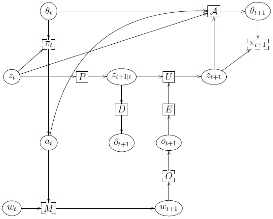
Figure 1.2: Detailed illustration of the interaction of an agent in an environment. The agent has internal state \(z_t\), and chooses action \(a_t\) based on its policy \(π_t\) using \(a_t \sim π_t(z_t|θ_t)\). It then predicts its next internal states, \(z_{t+1|t}\), via the predict function \(P\), and optionally predicts the resulting observation, \(\hat{o}_{t+1}\) , via the observation decoder \(D\). The environment has (hidden) internal state \(w_t\), which gets updated by the environment model \(M\) to give the new state \(w_{t+1} ∼ M(w_t, a_t)\) in response to the agent's action. The environment also emits an observation \(o_{t+1}\) via its observation model, \(o_{t+1} \sim O(w_{t+1})\). This gets encoded to \(e_{t+1} = E(o_{t+1})\) by the agent's observation encoder \(E\), which the agent uses to update its internal state using \(z_{t+1} = U(z_t, a_t, e_{t+1})\). The policy is parameterized by \(θ_t\), and these parameters may be updated (at a slower time scale) by an RL algorithm denoted by \(A\). Square nodes are functions, circles are variables (either random or deterministic), dashed square nodes are stochastic functions that take an extra source of randomness (not shown).
図1.2: 環境におけるエージェントの相互作用の詳細図。エージェントは内部状態\(z_t\)を持ち、ポリシー\(π_t\)に基づいて\(a_t \sim π_t(z_t|θ_t)\)を用いて行動\(a_t\)を選択する。次に、予測関数\(P\)を介して次の内部状態\(z_{t+1|t}\)を予測し、オプションで観測デコーダー\(D\)を介して結果の観測値\(\hat{o}_{t+1}\)を予測する。環境には(隠れた)内部状態\(w_t\)があり、これは環境モデル\(M\)によって更新され、エージェントの行動に応じて新しい状態\(w_{t+1} ∼ M(w_t, a_t)\)となる。環境はまた、観測モデル \(o_{t+1} \sim O(w_{t+1})\) を介して観測 \(o_{t+1}\) を出力します。これは、エージェントの観測エンコーダ \(E\) によって \(e_{t+1} = E(o_{t+1})\) にエンコードされ、エージェントはこれを使用して、\(z_{t+1} = U(z_t, a_t, e_{t+1})\) を使用して内部状態を更新します。ポリシーは \(θ_t\) によってパラメーター化され、これらのパラメーターは、\(A\) で示される RL アルゴリズムによって(より遅い時間スケールで)更新される場合があります。四角いノードは関数、円は変数(ランダムまたは決定論的)、破線の四角いノードは、追加のランダム性ソース(図示せず)を取る確率関数です。
Thus the agent needs use these observations to main an internal belief state about the world, denoted by \(z\). This gets updated using the state update function
したがって、エージェントはこれらの観察結果を用いて、世界に関する内部の信念状態(\(z\) で示される)を維持する必要がある。これは状態更新関数によって更新される。
\[
z_{t+1} = SU(z_t, a_t, o_{t+1}) \tag{1.10}
\]
In the simplest setting, the internal \(z_t\) can just store all the past observations, \(\mathbf{h}_t = (\mathbf{o}_{1:t},\mathbf{a}_{1:t−1})\), but such non-parametric models can take a lot of time and space to work with, so we will usually consider parametric approximations. The agent can then pass its state to its policy to pick actions, using \(a_{t+1} = π_t(z_{t+1})\).
最も単純な設定では、内部の\(z_t\)は過去のすべての観測値(\(\mathbf{h}_t = (\mathbf{o}_{1:t},\mathbf{a}_{1:t−1})\))を保存できますが、このような非パラメトリックモデルは処理に多くの時間と空間を要するため、通常はパラメトリック近似を検討します。エージェントは、\(a_{t+1} = π_t(z_{t+1})\)を使用して、状態をポリシーに渡してアクションを選択できます。
We can further elaborate the behavior of the agent by breaking the state-update function into two parts. First the agent predicts its own next state, \(z_{t+1|t} = P(z_t, a_t)\), using a prediction function \(P\), and then it updates this prediction given the observation using update function \(U\), to give \(z_{t+1} = U(z_{t+1|t}, o_{t+1})\). Thus the \(SU\) function is defined as the composition of the predict and update functions
状態更新関数を2つの部分に分割することで、エージェントの行動をさらに詳細に説明することができます。まず、エージェントは予測関数 \(P\)を用いて自身の次の状態 \(z_{t+1|t} = P(z_t, a_t)\) を予測し、次に更新関数 \(U\)を用いて観測値に基づいてこの予測を更新し、\(z_{t+1} = U(z_{t+1|t}, o_{t+1})\) とします。このように、\(SU\)関数は予測関数と更新関数の合成として定義されます。
\[
z_{t+1} = U(P(z_t, a_t), o_{t+1}) \tag{1.11}
\]
If the observations are high dimensional (e.g., images), the agent may choose to encode its observations into a low-dimensional embedding \(e_{t+1}\) using an encoder, \(e_{t+1} = E(o_{t+1})\); this can encourage the agent to focus on the relevant parts of the sensory signal. In this case, the state update becomes
観測が高次元(例えば画像)である場合、エージェントはエンコーダを用いて観測を低次元埋め込み\(e_{t+1}\)にエンコードすることを選択するかもしれない(\(e_{t+1} = E(o_{t+1})\)。これにより、エージェントは感覚信号の関連部分に集中するようになる。この場合、状態更新は次のようになる。
\[
z_{t+1} = U(P(z_t, a_t), E(o_{t+1})) \tag{1.12}
\]
Optionally the agent can also learn to invert this encoder by training a decoder to predict the next observation using \(\hat{o}_{t+1} = D(z_{t+1|t})\); this can be a useful training signal, as we will discuss in Chapter
4. Finally, the agent needs to learn the action policy \(π_t(z_t) = π(z_t;\mathbf{θ}_t)\). We can update the policy parameters using a learning algorithm, denoted
オプションとして、エージェントは、デコーダーを訓練して次の観測を\(\hat{o}_{t+1} = D(z_{t+1|t})\)を用いて予測することで、このエンコーダーを反転させることも学習できます。これは、第4章で説明するように、有用な訓練信号となります。最後に、エージェントは行動ポリシー\(π_t(z_t) = π(z_t;\mathbf{θ}_t)\)を学習する必要があります。ポリシーパラメータは、学習アルゴリズムを用いて更新できます。
\[
\mathbf{θ}_t = \mathcal{A}(o_{1:t}, a_{1:t}, r_{1:t}) =
\mathcal{A}(\mathbf{θ}_{t−1}, a_t, z_t, r_t) \tag{1.13}
\]
See Figure 1.2 for an illustration.
図説は図 1.2 を参照してください。
We see that, in general, there are three interacting stochastic processes we need to deal with: the environment's states \(w_t\) (which are usually affected by the agents actions); the agent's internal states \(z_t\) (which reflect its beliefs about the environment based on the observed data); and the agent's policy parameters \(\mathbf{θ}_t\) (which are updated based on the information stored in the belief state and the external observations).
一般的に、対処する必要がある相互作用する確率過程が 3 つあることがわかります。環境の状態 \(w_t\) (通常はエージェントのアクションによって影響を受けます)、エージェントの内部状態 \(z_t\) (観測データに基づいて環境に関する信念を反映)、エージェントのポリシー パラメーター \(\mathbf{θ}_t\) (信念状態に格納された情報と外部観測に基づいて更新されます) です。
In later chapters, we will describe methods for learning the best policy to maximize Vπ(s0) = E[G0|s0, π]). More details on RL can be found in textbooks such as [SB18 ; KWW22 ; Pla22 ; Li23 ; Sze10], and reviews such as [Aru+17 ; FL+18 ; Li18 ; Wen18a ; ID19]. For a more theoretical treatment, see e.g., [Aga+22a; MMT24 ; FR23]. For details on how RL relates to control theory , see e.g., [Son98; Rec19; Ber19 ; Mey22]; for connections to operations research, see [Pow22]; for connections to finance, see [RJ22].
後の章では、Vπ(s0) = E[G0|s0, π]) を最大化する最適なポリシーを学習する方法について説明します。強化学習の詳細については、[SB18 ; KWW22 ; Pla22 ; Li23 ; Sze10] などの教科書や、[Aru+17 ; FL+18 ; Li18 ; Wen18a ; ID19] などのレビューを参照してください。より理論的な処理については、例えば [Aga+22a; MMT24 ; FR23] を参照してください。強化学習と制御理論の関係の詳細については、例えば [Son98; Rec19; Ber19 ; Mey22] を参照してください。オペレーションズリサーチとの関連については [Pow22] を、ファイナンスとの関連については [RJ22] を参照してください。
In this section, we describe different forms of model for the environment and the agent that have been studied in the literature.
このセクションでは、文献で研究されてきた環境とエージェントのさまざまな形式のモデルについて説明します。
The model shown in Figure 1.2 is called a partially observable Markov decision process or POMDP (pronounced “pom-dee-pee”) [KLC98 ; LHP22 ; Sub+22]. Typically the environment's dynamics model is represented by a stochastic transition function, rather than a deterministic function with noise as an input. We can derive this transition function as follows:
図1.2に示すモデルは、部分観測マルコフ決定過程、またはPOMDP(「ポムディーピー」と発音)と呼ばれます[KLC98 ; LHP22 ; Sub+22]。一般的に、環境のダイナミクスモデルは、ノイズを入力とする決定論的関数ではなく、確率的遷移関数で表されます。この遷移関数は以下のように導出できます。
\[
p(w_{t+1}|w_t, a_t) = \mathbb{E}_{ε_t^w}[\mathbb{I}(w_{t+1}= W(w_t, a_t, ε_t^w
))] \tag{1.14}
\]
Similarly the stochastic observation function is given by
同様に確率的観測関数は次のように与えられる。
\[
p(o_{t+1} |w_{t+1} ) = \mathbb{E}_{ε_{t+1}^o}[\mathbb{I}(o_{t+1}= O(w_{t+1},ε_{t+1}^o))] \tag{1.15}
\]
Note that we can combine these two distributions to derive the joint world model \(p_{WO}(w_{t+1}, o_{t+1}|w_t, a_t)\). Also, we can use these distributions to derive the environment's non-Markovian observation distribution, \(p_{env}(o_{t+1}|o_{1:t}, a_{1:t})\), used in Equation (1.4), as follows:
これら2つの分布を組み合わせて、結合世界モデル\(p_{WO}(w_{t+1}, o_{t+1}|w_t, a_t)\)を導出できることに注意してください。また、これらの分布を使用して、式(1.4)で使用される環境の非マルコフ観測分布\(p_{env}(o_{t+1}|o_{1:t}, a_{1:t})\)を次のように導出できます。
\[
\begin{align}
p_{env}(o_{t+1}|o_{1:t}, a_{1:t}) &= \sum_{w_{t+1}}p(o_{t+1}|w_{t+1})p(w_{t+1}|a_{1:t}) \tag{1.16} \\
\\
p(w_{t+1}|a_{1:t}) &= \sum_{w_1}\cdots\sum_{w_t} p(w_1|a_1)p(w_2|w_1, a_1)\cdots
p(w_{t+1}|w_t, a_t) \tag{1.17}
\end{align}
\]
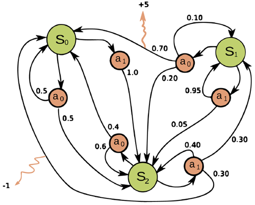
Figure 1.3: Illustration of an MDP as a finite state machine (FSM). The MDP has three discrete states (green cirlces), two discrete actions (orange circles), and two non-zero rewards (orange arrows). The numbers on the black edges represent state transition probabilities, e.g., \(p(s^\prime = s_0|a = a_0, s^\prime = s_1) = 0.7\); most state transitions are impossible (probability \(0\)), so the graph is sparse. The numbers on the yellow wiggly edges represent expected rewards, e.g., \(R(s = s_1, a = a_0, s^\prime = s_0) = +5\) ; state transitions with zero reward are not annotated. From https: // en. wikipedia. org/ wiki/ Markov_ decision_ process .
図1.3: 有限状態機械 (FSM) としての MDP の図。MDP には、3 つの離散状態 (緑の円)、2 つの離散アクション (オレンジ色の円)、および 2 つの非ゼロ報酬 (オレンジ色の矢印) があります。黒いエッジの数字は状態遷移確率を表します (例: \(p(s^\prime = s_0|a = a_0, s^\prime = s_1) = 0.7\)。ほとんどの状態遷移は不可能 (確率 \(0\)) であるため、グラフはスパースです。黄色の波状のエッジの数字は期待報酬を表します (例: \(R(s = s_1, a = a_0, s^\prime = s_0) = +5\)。報酬がゼロの状態遷移には注釈が付けられていません。出典: https://en.wikipedia.org/wiki/マルコフ決定過程。
If the world model (both \(p(o|w)\) and \(p(w^\prime|w, a ))\) is known, then we can — in principle — solve for the optimal policy. The method requires that the agent's internal state correspond to the belief state \(s_t = \mathbf{b}_t = p(w_t|\mathbf{h}_t)\), where \(\mathbf{h}_t = (o_{1:t}, a_{1:t−1})\) is the observation history. The belief state can be updated recursively using Bayes rule. See Section 1.2.6 for details. The belief state forms a sufficient statistic for the optimal policy. Unfortunately, computing the belief state and the resulting optimal policy is wildly intractable [PT87 ; KLC98]. We discuss some approximate methods in Section 1.3.4.
世界モデル(\(p(o|w)\)と\(p(w^\prime|w, a ))\)の両方が既知であれば、原理的には最適ポリシーを解くことができます。この方法では、エージェントの内部状態が信念状態 \(s_t = \mathbf{b}_t = p(w_t|\mathbf{h}_t)\) に対応している必要があります。ここで、\(\mathbf{h}_t = (o_{1:t}, a_{1:t−1})\)は観測履歴です。信念状態はベイズ則を用いて再帰的に更新できます。詳細は1.2.6節を参照してください。信念状態は最適ポリシーの十分な統計量となります。残念ながら、信念状態と結果として得られる最適ポリシーの計算は非常に困難です[PT87; KLC98]。1.3.4節でいくつかの近似手法について説明します。
A Markov decision process [Put94] is a special case of a POMDP in which the environment states are observed, so \(w_t = o_t = s_t\). We usually define an MDP in terms of the state transition matrix induced by the world model:
マルコフ決定過程 [Put94] は、環境状態が観測される POMDP の特殊なケースであり、\(w_t = o_t = s_t\) となります。MDP は通常、世界モデルによって誘導される状態遷移行列を用いて定義されます。
\[
p_S(s_{t+1}|s_t, a_t) = \mathbb{E}_{ε_t^s} [\mathbb{I}(s_{t+1} = W(s_t, a_t, ε_t^s))] \tag{1.18}
\]
In lieu of an observation model, we assume the environment (as opposed to the agent) sends out a reward signal, sampled from \(p_R(r_t|s_t, a_t, s_{t+1})\). The expected reward is then given by
観測モデルの代わりに、環境(エージェントではなく)が\(p_R(r_t|s_t, a_t, s_{t+1})\)からサンプリングされた報酬信号を送信すると仮定する。期待報酬は次のように与えられる。
\[
\begin{align}
R(s_t, a_t, s_{t+1}) &= \sum_r r p_R(r|s_t, a_t, s_{t+1}) \tag{1.19} \\
\\
R(s_t, a_t) &= \sum_{s_{t+1}} p_S(s_{t+1}|s_t, a_t)R(s_t, a_t, s_{t+1}) \tag{1.20}
\end{align}
\]
Note that the field of control theory uses slightly different terminology and notation when describing the same setup: the environment is called the plant , the agent is called the controller , States are denoted by \(x_t ∈ \mathcal{X} ⊆ \mathbb{R}^D\), actions are denoted by \(u_t ∈ \mathcal{U} ⊆ \mathbb{R}^K\), and rewards are replaced by costs \(c_t ∈ \mathbb{R}\).
制御理論の分野では、同じ設定を説明する際に、若干異なる用語と表記法を使用することに注意してください。環境は プラント と呼ばれ、エージェントは コントローラー と呼ばれ、状態は \(x_t ∈ \mathcal{X} ⊆ \mathbb{R}^D\) で表され、アクションは \(u_t ∈ \mathcal{U} ⊆ \mathbb{R}^K\) で表され、報酬はコスト \(c_t ∈ \mathbb{R}\) に置き換えられます。
Given a stochastic policy \)π(a_t|s_t)\), the agent can interact with the environment over many steps. Each step is called a transition , and consists of the tuple \((s_t, a_t, r_t, s_{t+1})\), where \(a_t \sim π(·| s_t), s_{t+1} \sim p_S(s_t, a_t)\), and \(r_t ∼ p_R(s_t, a_t, s_{t+1})\). Hence, under policy \(π\), the probability of generating a trajectory length \(T, \mathbb{τ} = (s_0, a_0, r_0, s_1, a_1, r_1, s_2, ..., s_T)\), can be written explicitly as
確率的方策 \)π(a_t|s_t)\) が与えられた場合、エージェントは環境と複数のステップにわたって相互作用することができます。各ステップは 遷移 と呼ばれ、タプル \((s_t, a_t, r_t, s_{t+1})\) で構成されます。ここで、 \(a_t \sim π(·| s_t), s_{t+1} \sim p_S(s_t, a_t)\)、および \(r_t ∼ p_R(s_t, a_t, s_{t+1})\) です。したがって、方策\(π\)の下で、長さ\(T, \mathbb{τ} = (s_0, a_0, r_0, s_1, a_1, r_1, s_2, ..., s_T)\)の軌道を生成する確率は、次のように明示的に表すことができます。
\[
p(\mathbf{τ}) = p_0(s_0)\prod_{t=0}^{T-1} π(a_t|s_t)p_S(s_{t+1}|s_t, a_t)p_R(r_t|s_t, a_t, s_{t+1}) \tag{1.21}
\]
In general, the state and action sets of an MDP can be discrete or continuous. When both sets are finite, we can represent these functions as lookup tables; this is known as a tabular representation . In this case, we can represent the MDP as a finite state machine , which is a graph where nodes correspond to states, and edges correspond to actions and the resulting rewards and next states. Figure 1.3 gives a simple example of an MDP with 3 states and 2 actions.
一般に、MDPの状態とアクションの集合は離散的または連続的です。両方の集合が有限の場合、これらの関数をルックアップテーブルとして表現できます。これは表形式表現と呼ばれます。この場合、MDPを有限ステートマシンとして表現できます。これは、ノードが状態に対応し、エッジがアクションとその結果としての報酬と次の状態に対応するグラフです。図1.3は、3つの状態と2つのアクションを持つMDPの簡単な例を示しています。
If we know the world model \(p_S\) and \(p_R\), and if the state and action space is tabular, then we can solve for the optimal policy using dynamic programming techniques, as we discuss in Section 2.2. However, typically the world model is unknown, and the states and actions may need complex nonlinear models to represent their transitions. In such cases, we will have to use RL methods to learn a good policy.
世界モデル \(p_S\) と \(p_R\) が既知であり、状態空間と行動空間が表形式である場合、2.2節で説明するように、動的計画法を用いて最適な方策を解くことができます。しかし、通常、世界モデルは未知であり、状態と行動の遷移を表現するために複雑な非線形モデルが必要になる場合があります。そのような場合、適切な方策を学習するために強化学習(RL)手法を使用する必要があります。
A goal-conditioned MDP is one in which the reward is defined as \(R(s, a|g) = 1\) iff the goal state is achieved, i.e., \(R(s, a|s) = \mathbb{I}(s = g)\). We can also define a dense reward signal using some state abstraction function \(\phi\), by definining \(R(s, a|g) = sim (s, g)\), where sim is some kind of similarity metric. For example, if \(s\) is an image and \(g\) is a sentence, we may use cosine similarity
目標条件付きMDPとは、目標状態が達成された場合に限り報酬が\(R(s, a|g) = 1\)と定義されるMDP、すなわち\(R(s, a|s) = \mathbb{I}(s = g)\)となるMDPです。また、状態抽象関数\(\phi\)を用いて、\(R(s, a|g) = sim (s, g)\)と定義することで、稠密な報酬信号を定義することもできます。ここで、simは類似度指標の一種です。例えば、\(s\)が画像で\(g\)が文の場合、コサイン類似度を使用することができます。
\[
sim (s,g) = \frac{\phi(s)^Tψ(g)}{||\phi(s)||\; ||ψ(g)||} \tag{1.22}
\]
where \(\phi(s)\) is an embedding of the image (state). and \(ψ(g)\) is an embedding of the text (goal). Such embeddings can be computed by using a VLM or vision-language model (see Section 6.2.2).
ここで、\(\phi(s)\)は画像(状態)の埋め込みであり、\(ψ(g)\)はテキスト(目標)の埋め込みです。このような埋め込みは、VLMまたは視覚言語モデルを用いて計算できます(6.2.2節を参照)。
A goal-conditioned policy of the form \(π(a|s, g)\) is sometimes called a universal policy [Sch+15a]. We can learn such policies using goal-conditioned RL methods (see e.g., [LZZ22] and Section 2.5.5).
\(π(a|s, g)\) という形式の目標条件付き方策は、普遍方策と呼ばれることもあります [Sch+15a]。このような方策は、目標条件付き強化学習法を用いて学習できます(例えば、[LZZ22] および2.5.5節を参照)。
Note that multi-goal RL is different to multi-task RL. The latter refers to the ability to solve different “tasks”, which correspond to entire MDPs (with different dynamics as well as different rewards).
マルチゴール強化学習はマルチタスク強化学習とは異なることに注意してください。後者は、MDP全体に対応する異なる「タスク」(異なるダイナミクスと異なる報酬を持つ)を解決する能力を指します。
A Contextual MDP [HDCM15] is an MDP where the dynamics and rewards of the environment depend on a hidden static parameter referred to as the context. (This is different to a contextual bandit, discussed in Section 1.2.5, where the context is observed at each step.) A simple example of a contextual MDP is a video game, where each level of the game is procedurally generated , that is, it is randomly generated each time the agent starts a new episode. Thus the agent must solve a sequence of related MDPs, which are drawn from a common distribution. This requires the agent to generalize across multiple MDPs, rather than overfitting to a specific environment [Cob+19 ; Kir+21; Tom+22]. (This form of generalization is different from generalization within an MDP, which requires generalizing across states, rather than across environments; both are important.)
コンテキスト MDP [HDCM15] は、環境のダイナミクスと報酬がコンテキストと呼ばれる隠れた静的パラメータに依存する MDP です。(これは、セクション 1.2.5 で説明した、各ステップでコンテキストが観測されるコンテキスト バンディットとは異なります。)コンテキスト MDP の簡単な例としては、ゲームの各レベルが 手続き的に生成 される、つまり、エージェントが新しいエピソードを開始するたびにランダムに生成されるビデオ ゲームがあります。したがって、エージェントは、共通の分布から抽出された一連の関連する MDP を解く必要があります。これには、エージェントが特定の環境に過剰適合するのではなく、複数の MDP に一般化する必要があります [Cob+19 ; Kir+21; Tom+22]。(この形式の一般化は、環境全体ではなく状態全体の一般化を必要とする MDP 内の一般化とは異なります。どちらも重要です。)
A contextual MDP is a special kind of POMDP where the hidden variable corresponds to the unknown parameters of the model. In [Gho+21], they call this an epistemic POMDP , which is closely related to the concept of belief state MDP which we discuss in Section 1.2.6.
文脈的MDPは、隠れ変数がモデルの未知のパラメータに対応する特殊なPOMDPです。[Gho+21]では、これを認識論的POMDPと呼んでおり、これは1.2.6節で議論する信念状態MDPの概念と密接に関連しています。
A contextual bandit is a special case of a POMDP where the world state transition function is independent of the action of the agent and the previous state, i.e., \(p(w_t|w_{t−1}, a_t) = p(w_t)\). In this case, we call the world states “contexts”; these are observable by the agent, i.e., \(o_t = w_t\). Since the world state distribution is independent of the agents actions, the agent has no effect on the external environment. However, its actions do affect the rewards that it receives. Thus the agent's internal belief state — about the underlying reward function \(R(o, a)\) — does change over time, as the agent learns a model of the world (see Section 1.2.6).
コンテキストバンディットは POMDP の特殊なケースであり、世界の状態遷移関数はエージェントの行動や以前の状態とは独立しています。つまり、\(p(w_t|w_{t−1}, a_t) = p(w_t)\) です。この場合、世界の状態を「コンテキスト」と呼びます。コンテキストはエージェントによって観測可能です。つまり、\(o_t = w_t\) です。世界の状態の分布はエージェントの行動とは独立しているため、エージェントは外部環境に影響を与えません。ただし、その行動はエージェントが受け取る報酬に影響を与えます。したがって、エージェントが世界のモデルを学習するにつれて、エージェントの内部的な信念状態 (基礎となる報酬関数 \(R(o, a)\) に関する) は時間の経過とともに変化します (セクション 1.2.6 を参照)。
A special case of a contextual bandit is a regular bandit, in which there is no context, or equivalently, st is some fixed constant that never changes. When there are a finite number of possible actions, \(\mathcal{A} = \{a_1, ..., a_K\}\), this is called a multi-armed bandit. 4 In this case the reward model has the form \(R(a) = f(w_a)\), where wa are the parameters for arm \(a\).
コンテキストバンディットの特殊なケースとして、コンテキストが存在しない通常のバンディット、つまりstが決して変化しない固定定数であるバンディットがあります。可能なアクションの数が有限である場合、\(\mathcal{A} = \{a_1, ..., a_K\}\)、これは多腕バンディットと呼ばれます。4 この場合、報酬モデルは\(R(a) = f(w_a)\)の形をとります。ここで、waはarm \(a\)のパラメータです。
4
The terminology arises by analogy to a slot machine (sometimes called a “bandit”, because it steals your money) in a casino. If there are K slot machines, each with different rewards (payout rates), then the agent (player) must explore the different machines (by pulling the arms) until they have discovered which one is best, and can then stick to exploiting it.
この用語は、カジノのスロットマシン(お金を盗むため「バンディット」と呼ばれることもあります)とのアナロジーから生まれました。K台のスロットマシンがあり、それぞれが異なる報酬(ペイアウト率)を持っているとします。エージェント(プレイヤー)は、どのマシンが最適かを見つけるまで(アームを引くことで)様々なマシンを探索し、その後はそれを使い続ける必要があります。
Contextual bandits have many applications. For example, consider an online advertising system . In this case, the state st represents features of the web page that the user is currently looking at, and the action at represents the identity of the ad which the system chooses to show. Since the relevance of the ad depends on the page, the reward function has the form \(R(s_t, a_t)\), and hence the problem is contextual. The goal is to maximize the expected reward, which is equivalent to the expected number of times people click on ads; this is known as the click through rate or CTR . (See e.g., [Gra+10 ; Li+10 ; McM+13 ; Aga+14; Du+21; YZ22] for more information about this application.) Another application of contextual bandits arises in clinical trials [VBW15]. In this case, the state st are features of the current patient we are treating, and the action at is the treatment the doctor chooses to give them (e.g., a new drug or a placebo).
コンテキストバンディットには多くの応用があります。たとえば、オンライン広告システムを考えてみましょう。この場合、状態 st はユーザーが現在閲覧しているウェブページの特徴を表し、アクション at はシステムが表示することを選択した広告の ID を表します。広告の関連性はページによって異なるため、報酬関数は \(R(s_t, a_t)\) の形式となり、したがって問題はコンテキスト依存となります。目標は期待報酬を最大化することです。期待報酬はユーザーが広告をクリックする期待回数に相当し、これは クリックスルー率 または CTR として知られています。(この応用に関する詳細は、[Gra+10 ; Li+10 ; McM+13 ; Aga+14; Du+21; YZ22] などを参照してください。) コンテキストバンディットのもう 1 つの応用は 臨床試験 [VBW15] です。この場合、状態 st は現在治療している患者の特徴であり、アクション at は医師が患者に選択する治療法 (新薬や プラセボなど) です。
For more details on bandits, see e.g., [LS19 ; Sli19].
バンディット問題の詳細については、例えば[LS19; Sli19]を参照してください。
In this section, we describe a kind of MDP where the state represents a probability distribution, known as a belief state or information state , which is updated by the agent (“in its head”) as it receives information from the environment. 5 More precisely, consider a contextual bandit problem, where the agent approximates the unknown reward by a function \(R(o, a) = f(o, a;\mathbf{w})\). Let us denote the posterior over the unknown parameters by \(\mathbf{b}_t = p(\mathbf{w}|\mathbf{h}_t)\), where \(\mathbf{h}_t = \{o_{1:t}, a_{1:t}, r_{1:t}\}\)
is the history of past observations, actions and rewards. This belief state can be updated deterministically using Bayes' rule; we denote this operation by \(\mathbf{b}_{t+1} = \text{
BayesRule} (\mathbf{b}_t, o_{t+1}, a_{t+1}, r_{t+1})\). (This corresponds to the state update \(SU\) defined earlier.) Using this, we can define the following belief state MDP , with deterministic dynamics given by
このセクションでは、状態が確率分布を表す一種の MDP について説明します。これは 信念状態 または 情報状態 と呼ばれ、エージェントが環境から情報を受け取ると(「頭の中で」)更新されます。 5 より正確には、エージェントが未知の報酬を関数 \(R(o, a) = f(o, a;\mathbf{w})\) で近似するコンテキスト バンディット問題を考えます。未知のパラメーターの事後分布を \(\mathbf{b}_t = p(\mathbf{w}|\mathbf{h}_t)\) で表します。ここで、 \(\mathbf{h}_t = \{o_{1:t}, a_{1:t}, r_{1:t}\}\) は過去の観測、アクション、報酬の履歴です。この信念状態はベイズの定理を用いて決定論的に更新することができる。この操作を\(\mathbf{b}_{t+1} = \text{BayesRule} (\mathbf{b}_t, o_{t+1}, a_{t+1}, r_{t+1})\)と記す。(これは先に定義した状態更新\(SU\)に対応する。)これを用いて、次の信念状態MDPを定義することができる。これは、決定論的ダイナミクスは次のように与えられる。
5
Technically speaking, this is a POMDP, where we assume the states are observed, and the parameters are the unknown hidden random variables. This is in contrast to Section 1.2.1 , where the states were not observed, and the parameters were assumed to be known.
技術的に言えば、これはPOMDPであり、状態は観測され、パラメータは未知の隠れ確率変数であると仮定します。これは、状態は観測されず、パラメータは既知であると仮定したセクション1.2.1とは対照的です。
\[
p(\mathbf{b}_{t+1}|\mathbf{b}_t, o_{t+1}, a_{t+1}, r_{t+1}) =
\mathbb{I}(\mathbf{b}_{t+1} = \text{BayesRule}(\mathbf{b}_t, o_{t+1}, a_{t+1}, r_{t+1})) \tag{1.23}
\]
and reward function given by
そして報酬関数は次のように与えられる。
\[
p(r_t|o_t, a_t,\mathbf{b}_t) = \int p_R(r_t|o_t, a_t;\mathbf{w})p(\mathbf{w}|\mathbf{b}_t)d\mathbf{w} \tag{1.24}
\]
If we can solve this (PO)MDP, we have the optimal solution to the exploration-exploitation problem (see Section 1.3.5).
この(PO)MDPを解くことができれば、探索・利用問題に対する最適解が得られます(セクション1.3.5を参照)。
As a simple example, consider a context-free Bernoulli bandit , where \(p_R(r|a) = Ber (r|µ_a)\), and \(µ_a = p_R(r = 1|a) = R(a)\) is the expected reward for taking action \(a\). The only unknown parameters are \(w = µ_{1:A}\). Suppose we use a factored beta prior
簡単な例として、文脈自由ベルヌーイバンディットを考えてみましょう。ここで、\(p_R(r|a) = Ber (r|µ_a)\)、\(µ_a = p_R(r = 1|a) = R(a)\)は、行動\(a\)を取った場合の期待報酬です。未知のパラメータは\(w = µ_{1:A}\)のみです。因数分解されたベータ事前分布を用いるとします。
\[
p_0(\mathbf{w}) = \prod_a \text{Beta}(µ_a|α_0^a, β_0^a) \tag{1.25}
\]
where \(\mathbf{w} = ( µ_1,..., µ_K)\). We can compute the posterior in closed form to get
ここで\(\mathbf{w} = ( µ_1,..., µ_K)\)である。事後分布を閉じた形で計算すると、
\[
p(\mathbf{w}|\mathcal{D}_t) = \prod_a \text{Beta}(µ_a|\underbrace{α_0^a +N_t^0(a)}_{α_t^0}, \underbrace{β_0^a+N_t^1(a)}_{β_t^a}) \tag{1.26}
\]
where
\[
N_t^r(a) = \sum_{i=1}^{t−1}\mathbb{I}(a_i = a, r_i= r) \tag{1.27}
\]
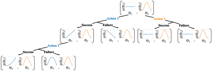
Figure 1.4: Illustration of sequential belief updating for a two-armed beta-Bernoulli bandit. The prior for the reward for action 1 is the (blue) uniform distribution Beta (1 ,1) ; the prior for the reward for action 2 is the (orange) unimodal distribution Beta (2 ,2) . We update the parameters of the belief state based on the chosen action, and based on whether the observed reward is success (1) or failure (0).
図1.4: 2本腕ベータベルヌーイバンディットにおける逐次的な信念更新の図解。行動1の報酬の事前分布は(青)一様分布Beta(1,1)であり、行動2の報酬の事前分布は(オレンジ)単峰分布Beta(2,2)である。選択された行動と、観測された報酬が成功(1)か失敗(0)かに基づいて、信念状態のパラメータを更新する。
This is illustrated in Figure 1.4 for a two-armed Bernoulli bandit. We can use a similar method for a Gaussian bandit , where \(p_R(r|a) = \mathcal{N}(r|µ_a, σ_a^2)\).
これは図1.4に2本腕のベルヌーイバンディットについて示されています。ガウスバンディットにも同様の手法を用いることができ、\(p_R(r|a) = \mathcal{N}(r|µ_a, σ_a^2)\)となります。
In the case of contextual bandits, the problem is conceptually the same, but becomes more complicated computationally. If we assume a linear regression bandit , \(p_R(r|s, a;\mathbf{w}) = \mathcal{N}(r|\phi(s, a)^T\mathbf{w}, σ^2)\), we can use Bayesian linear regression to compute \(p(\mathbf{w}|\mathcal{D}_t)\) exactly in closed form. If we assume a logistic regression bandit , \(pR(r|s, a;\mathbf{w}) = Ber (r|σ(\phi(s, a)^T\mathbf{w}))\) , we have to use approximate methods for approximate Bayesian logistic regression to compute \(p(\mathbf{w}|\mathcal{D}_t)\). If we have a neural bandit of the form \(p_R(r|s, a;\mathbf{w}) = \mathcal{N}(r|f(s, a ;\mathbf{w})\)) for some nonlinear function f, then posterior inference is even more challenging (this is equivalent to the problem of inference in Bayesian neural networks, see e.g., [Arb+23] for a review paper for the offline case, and [DMKM22 ; JCM24] for some recent online methods).
コンテキストバンディットの場合、問題は概念的には同じですが、計算がより複雑になります。線形回帰バンディット、\(p_R(r|s, a;\mathbf{w}) = \mathcal{N}(r|\phi(s, a)^T\mathbf{w}, σ^2)\) を仮定すると、ベイズ線形回帰を用いて \(p(\mathbf{w}|\mathcal{D}_t)\) を閉形式で正確に計算できます。 ロジスティック回帰バンディット、\(pR(r|s, a;\mathbf{w}) = Ber (r|σ(\phi(s, a)^T\mathbf{w}))\) を仮定する場合、近似ベイズロジスティック回帰の近似法を使用して \(p(\mathbf{w}|\mathcal{D}_t)\) を計算する必要があります。ある非線形関数 f に対して \(p_R(r|s, a;\mathbf{w}) = \mathcal{N}(r|f(s, a ;\mathbf{w})\)) という形式のニューラルバンディットがある場合、事後推論はさらに困難になります(これはベイズニューラルネットワークの推論の問題に相当します。例えば、オフラインの場合のレビュー論文については [Arb+23] を、最近のオンライン手法については [DMKM22 ; JCM24] を参照してください)。
We can generalize the above methods to compute the belief state for the parameters of an MDP in the obvious way, but modeling both the reward function and state transition function.
上記の方法を一般化して、報酬関数と状態遷移関数の両方をモデル化し、MDP のパラメータの信念状態を明白な方法で計算することができます。
Once we have computed the belief state, we can derive a policy with optimal regret using the methods like UCB (Section 7.2.3) or Thompson sampling (Section 7.2.2).
信念状態を計算したら、UCB(セクション7.2.3)やトンプソンサンプリング(セクション7.2.2)などの方法を使用して、最適な後悔を持つポリシーを導出できます。
The bandit problem is an example of a problem where the agent must interact with the world in order to collect information, but it does not otherwise affect the environment. Thus the agents internal belief state changes over time, but the environment state does not. 6 Such problems commomly arise when we are trying to optimize a fixed but unknown function R. We can “query” the function by evaluating it at different points (parameter values), and in some cases, the resulting observation may also include gradient information. The agent's goal is to find the optimum of the function in as few steps as possible.
7 We give some examples of this problem setting below.
バンディット問題は、エージェントが情報を収集するために世界と相互作用する必要があるものの、それ以外は環境に影響を与えない問題の例です。したがって、エージェントの内部的な信念状態は時間とともに変化しますが、環境の状態は変化しません。6 このような問題は、固定されているが未知の関数Rを最適化しようとするときによく発生します。関数を異なるポイント(パラメータ値)で評価することで「クエリ」することができ、場合によっては、結果として得られる観測値に勾配情報も含まれることがあります。エージェントの目標は、できるだけ少ないステップで関数の最適解を見つけることです。
7 以下に、この問題設定の例をいくつか示します。
6
In the contextual bandit problem, the environment state (context) does change, but not in response to the agent's actions. Thus \(p(o_t)\) is usually assumed to be a static distribution.
文脈バンディット問題では、環境状態(コンテキスト)は変化しますが、エージェントの行動に応じて変化することはありません。したがって、\(p(o_t)\)は通常、静的分布であると仮定されます。
7
If we only care about the final performance of the agent, we can try to minimize the simple regret , which is just the regret at the last step, namely \(l_T\). This is the difference between the function value we chose and the true optimum. Minimizing simple regret results in a problem known as pure exploration [BMS11], where the agent needs to interact with the environment to learn the underlying MDP; at the end, it can then solve for the resulting policy using planning methods (see Section 2.2 ). However, in general RL problems, it is more common to focus on the cumulative regret , also called the total regret or just the regret , which is defined as \(L_T\overset{\triangle}{=}\mathbb{E}\big[\sum_{t=1}^T l_t\big]\).
エージェントの最終的なパフォーマンスだけを気にするのであれば、最後のステップでの後悔、つまり \(l_T\) である 単純後悔 を最小化するように努めることができます。これは、選択した関数値と真の最適値との差です。単純後悔を最小化すると、純粋探索 [BMS11] と呼ばれる問題が生じます。この問題では、エージェントは環境と対話して基礎となる MDP を学習する必要があります。最後に、計画手法を使用して結果のポリシーを解くことができます (セクション 2.2 を参照)。ただし、一般的な RL 問題では、累積後悔 (合計後悔または単に後悔とも呼ばれます) に焦点を当てる方が一般的です。これは \(L_T\overset{\triangle}{=}\mathbb{E}\big[\sum_{t=1}^T l_t\big]\) と定義されます。
In the standard multi-armed bandit problem our goal is to maximize the sum of expected rewards. However, in some cases, the goal is to determine the best arm given a fixed budget of T trials; this variant is known as best-arm identification [ABM10]. Formally, this corresponds to optimizing the final reward criterion:
標準的な多腕バンディット問題では、期待報酬の合計を最大化することが目標となります。しかし、場合によっては、T回の試行回数という固定された予算のもとで最適な腕を決定することが目標となることもあります。この方法は最適腕識別と呼ばれています[ABM10]。正式には、これは最終報酬基準の最適化に相当します。
\[
V_{π,π_T}= \mathbb{E}_{p(a_{1:T} ,r_{1:T}|s_0,π)}\big[R(\hat{a})\big] \tag{1.28}
\]
where \(\hat{a} = π_T(a_{1:T}, r_{1:T})\) is the estimated optimal arm as computed by the terminal policy \(π_T\) applied to the sequence of observations obtained by the exploration policy π. This can be solved by a simple adaptation of the methods used for standard bandits.
ここで、\(\hat{a} = π_T(a_{1:T}, r_{1:T})\)は、探索ポリシーπによって得られた観測系列に終端ポリシー\(π_T\)を適用することで計算される推定最適アームです。これは、標準的なバンディット法に用いられる手法を単純に適応させることで解くことができます。
Bayesian optimization is a gradient-free approach to optimizing expensive blackbox functions. That is, we want to find
ベイズ最適化は、高価なブラックボックス関数を最適化するための勾配フリーのアプローチです。つまり、
\[
\mathbf{w}^∗ = arg\max\limits_{\mathbf{w}} R(\mathbf{w}) \tag{1.29}
\]
for some unknown function \(R\), where \(\mathbf{w} ∈ \mathbb{R}^N\), using as few actions (function evaluations of \(R\)) as possible. This is essentially an “infinite arm” version of the best-arm identification problem [Tou14], where we replace the discrete choice of arms \(a ∈ \{1,..., K\}\) with the parameter vector w ∈ RN. In this case, the optimal policy can be computed if the agent's state st is a belief state over the unknown function, i.e., \(s_t = p(R|\mathbf{h}_t)\). A common way to represent this distribution is to use Gaussian processes. We can then use heuristics like expected improvement, knowledge gradient or Thompson sampling to implement the corresponding policy, \(\mathbf{w}_t = π(s_t)\). For details, see e.g., [Gar23].
何らかの未知の関数 \(R\) に対して、\(\mathbf{w} ∈ \mathbb{R}^N\) を、可能な限り少ないアクション(\(R\) の関数評価)で求める。これは本質的には、ベストアーム識別問題 [Tou14] の「無限アーム」バージョンであり、アームの離散選択 \(a ∈ \{1,..., K\}\) をパラメータベクトル w ∈ RN に置き換えたものである。この場合、エージェントの状態 st が未知の関数上の信念状態、すなわち \(s_t = p(R|\mathbf{h}_t)\) であれば、最適なポリシーを計算できる。この分布を表す一般的な方法は、ガウス過程を使用することである。そして、期待改善率、知識勾配、トンプソンサンプリングなどのヒューリスティックを用いて、対応するポリシー\(\mathbf{w}_t = π(s_t)\)を実装することができます。詳細については、[Gar23]等を参照してください。
Active learning is similar to BayesOpt, but instead of trying to find the point at which the function is largest (i.e., \(\mathbf{w}^∗\)), we are trying to learn the whole function \(R\), again by querying it at different points wt. Once again, the optimal strategy again requires maintaining a belief state over the unknown function, but now the best policy takes a different form, such as choosing query points to reduce the entropy of the belief state. See e.g., [Smi+23].
能動学習はBayesOptに似ていますが、関数が最大となる点(つまり\(\mathbf{w}^∗\))を探すのではなく、関数\(R\)全体を学習しようとします。この場合も、異なる点wtでクエリを実行することで学習します。ここでも最適な戦略は、未知の関数に対する確信状態を維持することを必要としますが、最適なポリシーは、確信状態のエントロピーを低減するようにクエリ点を選択するなど、異なる形をとります。例えば、[Smi+23]を参照してください。
Finally we discuss how to interpret SGD as a sequential decision making process, following [Pow22]. The action space consists of querying the unknown function R at locations \(\mathbf{a}_t = \mathbf{w}_t\), and observing the function value \(r_t = R(\mathbf{w}_t)\); however, unlike BayesOpt, now we also observe the corresponding gradient \(\mathbf{g}_t = ∇_{\mathbf{w}}R(\mathbf{w})|_{\mathbf{w}_t\), which gives non-local information about the function. The environment state contains the true function \(R\) which is used to generate the observations given the agent's actions. The agent state contains the current parameter estimate \(\mathbf{w}_t\), and may contain other information such as first and second moments \(\mathbf{m}_t\) and \(\mathbf{v}_t\), needed by methods such as Adam. The update rule (for vanilla SGD) takes the form \(\mathbf{w}_{t+1} = \mathbf{w}_t + α_t\mathbf{g}_t\), where the stepsize \(α_t\) is chosen by the policy, \(α_t = π(s_t)\). The terminal policy has the form \(π(s_T) = \mathbf{w}_T\).
最後に、[Pow22]に従って、SGDを順次的な意思決定プロセスとして解釈する方法について説明します。アクション空間は、場所\(\mathbf{a}_t = \mathbf{w}_t\)で未知の関数Rを照会し、関数値\(r_t = R(\mathbf{w}_t)\)を観測することで構成されます。ただし、BayesOptとは異なり、関数に関する非局所的な情報を提供する対応する勾配\(\mathbf{g}_t = ∇_{\mathbf{w}}R(\mathbf{w})|_{\mathbf{w}_t\)も観測します。環境状態には、エージェントのアクションが与えられた場合に観測値を生成するために使用される真の関数\(R\)が含まれます。エージェント状態には、現在のパラメータ推定値 \(\mathbf{w}_t\) が含まれます。また、Adamなどの手法で必要な、第1および第2モーメント \(\mathbf{m}_t\) や \(\mathbf{v}_t\) などの情報も含まれる場合があります。更新規則(バニラSGDの場合)は \(\mathbf{w}_{t+1} = \mathbf{w}_t + α_t\mathbf{g}_t\) の形式を取ります。ここで、ステップサイズ \(α_t\) はポリシー \(α_t = π(s_t)\) によって選択されます。最終ポリシーは \(π(s_T) = \mathbf{w}_T\) の形式を取ります。
Although in principle it is possible to learn the learning rate (stepsize) policy using RL (see e.g., [Xu+17]), the policy is usually chosen by hand, either using a learning rate schedule or some kind of manually designed adaptive learning rate policy (e.g., based on second order curvature information).
原理的にはRLを使って学習率(ステップサイズ)ポリシーを学習することは可能ですが(例えば[Xu+17]を参照)、ポリシーは通常、学習率スケジュールか、何らかの手動で設計された適応学習率ポリシー(例えば2次曲率情報に基づく)のいずれかを使用して手動で選択されます。
In this section, we give a brief overview of how to compute optimal policies when the model of the environment is unknown; this is the core problem tackled by RL. We mostly focus on the MDP case, but discuss the POMDP case in Section 1.3.4.
このセクションでは、環境モデルが未知の場合に最適なポリシーを計算する方法について簡単に概説します。これは強化学習が取り組む中核的な問題です。主にMDPの場合に焦点を当てますが、POMDPの場合については1.3.4節で説明します。
We can categorize RL methods along mutiple dimensions, such as the following:
RL 手法は、次のように複数の次元に沿って分類できます。
Table 1.1 lists a few common examples of RL methods, classified along these lines. More details are given in the subsequent sections.
\[
\begin{array}{l l l l l}
\text{Approach} & \text{Method} & \text{Functions learned} & \text{On/Off} & \text{Section} \\
\hline
\text{Value-based} & \text{SARSA} & Q(s, a ) & \text{On} & \text{Section 2.4} \\
\text{Value-based} & \text{Q-learning} & Q(s, a )& \text{Off} & \text{Section 2.5} \\
\hline
\text{Policy-based} & \text{REINFORCE} & π(a|s) & \text{On} & \text{Section 3.1.3} \\
\text{Policy-based} & \text{A2C} & π(a|s), V(s) & \text{On} & \text{Section 3.2.1} \\
\text{Policy-based} & \text{TRPO/PPO} & π(a|s), Adv (s, a ) & \text{On} & \text{Section 3.3.3} \\
\text{Policy-based} & \text{DDPG} & a = π(s), Q(s, a ) & \text{Off} & \text{Section 3.2.6.2} \\
\text{Policy-based} & \text{Soft actor-critic} & π(a|s), Q(s, a ) & \text{Off} & \text{Section 3.6.8} \\
\hline
\text{Model-based} & \text{MBRL} & p(s^\prime|s, a ) & \text{Off} & \text{Chapter 4}
\end{array}
\]
Table 1.1: Summary of some popular methods for RL. On/off refers to on-policy vs off-policy methods.
表1.1: 強化学習でよく使われる手法の概要。オン/オフは、オンポリシー手法とオフポリシー手法を表します。
In this section, we give a brief introduction to value-based RL , also called Approximate Dynamic Programming or ADP ; see Chapter 2 for more details.
このセクションでは、近似動的計画法 または ADP とも呼ばれる 価値ベース RL について簡単に説明します。詳細については、第 2 章を参照してください。
We introduced the value function Vπ(s) in Equation ( 1.1), which we repeat here for convenience:
式(1.1)で価値関数Vπ(s)を導入したが、便宜上ここでもこれを繰り返す。
\[
V_π(s)\overset{\triangle}{=}\mathbb{E}_π[G_0|s_0 = s] = \mathbb{E}_π\Bigg[\sum_{t=0}^\infty γ^t r_t|s_0=s\Bigg] \tag{1.30}
\]
The value function for the optimal policy \(π^∗\) is known to satisfy the following recursive condition, known as
Bellman's equation :
最適政策 \(π^∗\) の価値関数は、以下の再帰条件を満たすことが知られており、
ベルマン方程式として知られています。
\[
V^∗(s) = \max\limits_a R(s, a)+γ\mathbb{E}_{p_S(s^\prime|s,a)}[V^∗(s^\prime)] \tag{1.31}
\]
This follows from the principle of dynamic programming , which computes the optimal solution to a problem (here the value of state \(s\)) by combining the optimal solution of various subproblems (here the values of the next states \(s^\prime\)). This can be used to derive the following learning rule:
これは動的計画法の原理に従うもので、これは様々な部分問題の最適解(ここでは次の状態\(s^\prime\)の値)を組み合わせることで、問題(ここでは状態\(s\)の値)の最適解を計算するものです。これを用いて、以下の学習則を導き出すことができます。
\[
V(s) ← V (s) + η[r + γV (s^\prime) − V (s)] \tag{1.32}
\]
where \(s^\prime \sim p_S(·|s, a)\) is the next state sampled from the environment, and \(r = R(s, a)\) is the observed reward.
This is called Temporal Difference or TD learning (see Section 2.3.2 for details). Unfortunately, it is not
clear how to derive a policy if all we know is the value function. We now describe a solution to this problem.
ここで、\(s^\prime \sim p_S(·|s, a)\) は環境からサンプリングされた次の状態、\(r = R(s, a)\) は観測された報酬です。
これは時間差分学習またはTD学習と呼ばれます(詳細は2.3.2節を参照)。残念ながら、価値関数しか分かっていない場合、どのように方策を導出するかは明確ではありません。ここでは、この問題の解決策を説明します。
We first generalize the notion of value function to assigning a value to a state and action pair, by defining the Q function as follows:
まず、次のように Q 関数 を定義して、状態とアクションのペアに値を割り当てるという価値関数の概念を一般化します。
\[
Q_π(s,a)\overset{\triangle}{=}\mathbb{E}_π[G_0|s_0=s, a_0=a]=\mathbb{E}_π\Bigg[\sum_{t=0}^\infty γ^t r_t|s_0=s,a_0=a\Bigg] \tag{1.33}
\]
This quantity represents the expected return obtained if we start by taking action \(a\) in state \(s\), and then follow \(π\) to choose actions thereafter. The Q function for the optimal policy satisfies a modified Bellman equation
この量は、状態\(s\)において行動\(a\)から開始し、その後\(π\)に従って行動を選択する場合に得られる期待収益を表す。最適方策のQ関数は、修正ベルマン方程式を満たす。
\[
Q^∗(s, a) = R(s, a) + γ\mathbb{E}_{p_S(s^\prime|s,a)}\Big[\max\limits_{a^\prime} Q^∗(s^\prime, a^\prime)\Big] \tag{1.34}
\]
This gives rise to the following TD update rule:
これにより、次の TD 更新ルールが生成されます。
\[
Q(s,a) ← r + γ \max\limits_{a^\prime}Q(s^\prime, a^\prime)− Q(s,a) \tag{1.35}
\]
where we sample \(s^\prime \sim p_S(·|s, a)\) from the environment. The action is chosen at each step from the implicit policy
ここで、環境から\(s^\prime \sim p_S(·|s, a)\)をサンプリングする。各ステップで、暗黙のポリシーから行動が選択される。
\[
a = arg\max\limits_{a^\prime} Q(s, a^\prime) \tag{1.36}
\]
This is called Q learning (see Section 2.5 for details),
これはQ学習と呼ばれます(詳細はセクション2.5を参照)。
In this section we give a brief introductin to Policy-based RL ; for details see Chapter 3.
このセクションでは、ポリシーベース RL について簡単に説明します。詳細については、第 3 章を参照してください。
In policy-based methods, we try to directly maximize \(J(π_{\mathbf{θ}}) = \mathbb{E}_{p(s_0)}[V_π(s_0)]\) wrt the parameter's \(\mathbf{θ}\); this is called policy search . If \(J(π_{\mathbf{θ}}\) is differentiable wrt \(\mathbf{θ}\), we can use stochastic gradient ascent to optimize \(\mathbf{θ}\), which is known as policy gradient (see Section 3.1).
ポリシーベースの手法では、パラメータの\(\mathbf{θ}\)に関して\(J(π_{\mathbf{θ}}) = \mathbb{E}_{p(s_0)}[V_π(s_0)]\)を直接最大化しようとします。これはポリシー探索と呼ばれます。\(J(π_{\mathbf{θ}}\)が\(\mathbf{θ}\)に関して微分可能な場合、確率的勾配上昇法を使用して\(\mathbf{θ}\)を最適化できます。これはポリシー勾配と呼ばれます(セクション3.1を参照)。
Policy gradient methods have the advantage that they provably converge to a local optimum for many common policy classes, whereas Q-learning may diverge when approximation is used (Section 2.5.2.5). In addition, policy gradient methods can easily be applied to continuous action spaces, since they do not need to compute \(arg\max_a Q(s, a )\). Unfortunately, the score function estimator for \(∇_{\mathbf{θ}}J(π_{\mathbf{θ}})\) can have a very high variance, so the resulting method can converge slowly.
方策勾配法は、多くの一般的な方策クラスにおいて局所最適解に収束することが証明できるという利点がある一方、Q学習は近似値を用いると発散する可能性があります(セクション2.5.2.5)。さらに、方策勾配法は\(arg\max_a Q(s, a )\)を計算する必要がないため、連続行動空間に容易に適用できます。しかしながら、\(∇_{\mathbf{θ}}J(π_{\mathbf{θ}})\)のスコア関数推定値は非常に高い分散を持つ可能性があるため、結果として得られる手法の収束は遅くなる可能性があります。
One way to reduce the variance is to learn an approximate value function, \(V_{\mathbf{w}}(s)\), and to use it as a baseline in the score function estimator. We can learn \(V_{\mathbf{w}}(s)\) using using TD learning. Alternatively, we can learn an advantage function, \(A_{\mathbf{w}}(s, a )\), and use it as a baseline. These policy gradient variants are called actor critic methods, where the actor refers to the policy \(π_{\mathbf{θ}}\) and the critic refers to \(V_{\mathbf{w}}\) or \(A_{\mathbf{w}}\). See Section 3.2 for details.
分散を減らす1つの方法は、近似値関数 \(V_{\mathbf{w}}(s)\) を学習し、それをスコア関数推定値のベースラインとして使用することです。TD学習を用いて \(V_{\mathbf{w}}(s)\) を学習できます。あるいは、アドバンテージ関数 \(A_{\mathbf{w}}(s, a )\) を学習し、それをベースラインとして使用することもできます。これらのポリシー勾配の変種はアクター・クリティック法と呼ばれ、アクターはポリシー \(π_{\mathbf{θ}}\) を参照し、クリティックは \(V_{\mathbf{w}}\) または \(A_{\mathbf{w}}\) を参照します。詳細はセクション3.2を参照してください。
In this section, we give a brief introduction to model-based RL ; for more details, see Chapter 4.
このセクションでは、モデルベース RL について簡単に説明します。詳細については、第 4 章を参照してください。
Value-based methods, such as Q-learning, and policy search methods, such as policy gradient, can be very sample inefficient , which means they may need to interact with the environment many times before finding a good policy, which can be problematic when real-world interactions are expensive. In model-based RL, we first learn the MDP, including the \(p_S(s^\prime|s, a )\) and \(R(s, a )\) functions, and then compute the policy, either using approximate dynamic programming on the learned model, or doing lookahead search. In practice, we often interleave the model learning and planning phases, so we can use the partially learned policy to decide what data to collect, to help learn a better model.
Q 学習などの価値ベースの手法や、ポリシー勾配などのポリシー検索手法は、非常にサンプル効率が悪い 場合があります。つまり、適切なポリシーを見つけるまでに何度も環境とやり取りする必要がある場合があり、現実世界でのやり取りがコストがかかる場合には問題になる可能性があります。モデルベース RL では、最初に \(p_S(s^\prime|s, a )\) 関数と \(R(s, a )\) 関数を含む MDP を学習し、次に学習したモデルに対して近似動的計画法を使用するか、先読み検索を行ってポリシーを計算します。実際には、モデルの学習フェーズと計画フェーズをインターリーブすることが多く、部分的に学習したポリシーを使用して収集するデータを決定し、より良いモデルを学習できるようにします。
In an MDP, we assume that the state of the environment \(s_t\) is the same as the observation \(o_t\) obtained by the agent. But in many problems, the observation only gives partial information about the underlying state of the world (e.g., a rodent or robot navigating in a maze). This is called partial observability . In this case, using a policy of the form \(a_t = π(o_t)\) is suboptimal, since ot does not give us complete state information. Instead we need to use a policy of the form \(a_t = π(\mathbf{h}_t)\), where \(\mathbf{h}_t = (a_1, o_1,..., a_{t−1}, o_t)\) is the entire past history of observations and actions, plus the current observation. Since depending on the entire past is not tractable for a long-lived agent, various approximate solution methods have been developed, as we summarize below.
MDPでは、環境の状態 \(s_t\) はエージェントが取得した観測 \(o_t\) と同じであると仮定します。しかし多くの問題では、観測は世界の根本的な状態について部分的な情報しか提供しません(例:迷路を進むげっ歯類やロボット)。これは部分観測可能性と呼ばれます。この場合、 \(a_t = π(o_t)\) という形式のポリシーを使用するのは、ot では完全な状態情報が得られないため、最適ではありません。代わりに、 \(a_t = π(\mathbf{h}_t)\) という形式のポリシーを使用する必要があります。ここで、 \(\mathbf{h}_t = (a_1, o_1,..., a_{t−1}, o_t)\) は過去の観測と行動の履歴全体と、現在の観測です。長寿命エージェントの場合、過去全体に依存するのは扱いにくいため、以下にまとめるように、さまざまな近似解法が開発されています。
If we know the true latent structure of the world (i.e., both \(p(o|z)\) and \(p(z^\prime|z, a )\), to use the notation of Section 1.1.3), then we can use solution methods designed for POMDPs, discussed in Section 1.2.1 . This requires using Bayesian inference to compute a belief state, bt = p(wt|ht) (see Section 1.2.6), and then using this belief state to guide our decisions. However, learning the parameters of a POMDP (i.e., the generative latent world model) is very difficult, as is recursively computing and updating the belief state, as is computing the policy given the belief state. Indeed, optimally solving POMDPs is known to be computationally very difficult for any method [PT87 ; KLC98]. So in practice simpler approximations are used. We discuss some of these below. (For more details, see [Mur00].)
世界の真の潜在構造(つまり、セクション 1.1.3 の表記法を使用すると、 \(p(o|z)\) と \(p(z^\prime|z, a )\) の両方)がわかっていれば、セクション 1.2.1 で説明した POMDP 用に設計された解決方法を使用できます。これには、ベイズ推論を使用して信念状態 bt = p(wt|ht) を計算し(セクション 1.2.6 を参照)、この信念状態を使用して決定を導く必要があります。ただし、POMDP(つまり、生成潜在世界モデル)のパラメーターを学習することは非常に困難であり、信念状態を再帰的に計算して更新することや、信念状態が与えられたポリシーを計算することも同様です。実際、POMDP を最適に解くことは、どの方法でも計算的に非常に困難であることが知られています [PT87 ; KLC98]。そのため、実際にはより単純な近似が使用されます。以下では、これらのいくつかについて説明します。 (詳細は[Mur00]を参照)
Note that it is possible to marginalize out the POMDP latent state wt, to derive a prediction over the next observable state, \(p(o_{t+1} |\mathbf{h}_t,\mathbf{a}_t)\). This can then become a learning target for a model, that is trained to directly predict future observations, without explicitly invoking the concept of latent state. This is called a predictive state representation or PSR [LS01]. This is related to the idea of observable operator models [Jae00], and to the concept of successor representations which we discuss in Section 4.5.2.
POMDP潜在状態wtを周辺化して、次の観測可能な状態\(p(o_{t+1} |\mathbf{h}_t,\mathbf{a}_t)\)の予測を導くことが可能であることに留意されたい。これは、潜在状態の概念を明示的に呼び出すことなく、将来の観測を直接予測するように訓練されるモデルの学習目標となる。これは予測状態表現またはPSR [LS01]と呼ばれる。これは観測可能演算子モデル [Jae00]の考え方や、4.5.2節で説明する後継表現の概念に関連している。
The simplest solution to the partial observability problem is to define the state to be a finite history of the last k observations, \(s_t = \mathbf{h}_{t−k:t}\); when the observations ot are images, this is often called frame stacking . We can then use standard MDP methods. Unfortunately, this cannot capture long-range dependencies in the data.
部分観測可能性問題に対する最も単純な解は、状態を過去k回の観測の有限履歴\(s_t = \mathbf{h}_{t−k:t}\)と定義することです。観測データが画像の場合、これはしばしばフレームスタッキングと呼ばれます。この場合、標準的なMDP手法を使用できます。残念ながら、この方法ではデータ内の長距離依存性を捉えることができません。
A more powerful approach is to use a stateful policy, that can remember the entire past, and not just respond to the current input or last k frames. For example, we can represent the policy by an RNN (recurrent neural network), as proposed in the R2D2 paper [Kap+18], and used in many other papers. Now the hidden state wt of the RNN will implicitly summarize the past observations, ht, and can be used in lieu of the state st in any standard RL algorithm.
より強力なアプローチは、現在の入力や過去kフレームだけでなく、過去全体を記憶できる状態のあるポリシーを用いることです。例えば、R2D2論文[Kap+18]で提案され、他の多くの論文でも使用されているように、ポリシーをRNN(リカレントニューラルネットワーク)で表現することができます。RNNの隠れ状態wtは過去の観測値htを暗黙的に要約し、標準的な強化学習アルゴリズムの状態stの代わりに使用できます。
RNNs policies are widely used, and this method is often effective in solving partially observed problems. However, they typically will not plan to perform information-gathering actions, since there is no explicit notion of belief state or uncertainty. However, such behavior can arise via meta-learning [Mik+20].
RNNのポリシーは広く利用されており、この手法は部分観測問題の解決に効果的であることが多い。しかし、信念状態や不確実性といった明示的な概念がないため、通常は情報収集行動を計画することはない。しかし、メタ学習によってそのような行動が生じる可能性がある[Mik+20]。
In RL problems, we typically assume the underlying transition and reward models are not known. We can either try to explicitly learn these models (as in model-based RL), and then solve for the policy, or just learn the policy directly (as in model-free RL). But in either case, we need to explore the environment in order to collect enough data to figure out what to do. This may involve choosing between actions that the agent knows will yield high reward, vs choosing actions which might not been known to yield high reward but which will be informative about potential future gains. This is called the exploration-exploitation tradeoff . In this section, we discuss some simple heuristic solutions to this problem. See Section 7.2 for more sophisticated methods.
強化学習(RL)の問題では、通常、基盤となる遷移モデルと報酬モデルは未知であると仮定します。これらのモデルを明示的に学習して(モデルベースRLのように)、方策を解くことも、方策を直接学習することもできます(モデルフリーRLのように)。しかし、どちらの場合でも、何をすべきかを判断するのに十分なデータを収集するために、環境を探索する必要があります。これには、エージェントが高い報酬をもたらすとわかっている行動と、高い報酬をもたらすとはわかっていないかもしれないが、将来の潜在的な利益に関する情報となる行動のどちらかを選択することが含まれる場合があります。これは探索と活用のトレードオフと呼ばれます。このセクションでは、この問題に対するいくつかの簡単なヒューリスティックな解決策について説明します。より高度な方法については、セクション7.2を参照してください。
If we just want to exploit our current knowledge (without trying to learn new things), we can use the greedy policy:
新しいことを学ぼうとせずに、現在の知識を活用したいだけなら、貪欲ポリシー を使用できます。
\[
a_t = arg\max\limits_{a} Q(s, a ) \tag{1.37}
\]
We can add exploration to this by sometimes picking some other, non-greedy action, as we discuss below.
以下で説明するように、貪欲でない他のアクションを選択することで、これに探索を追加できます。
One approach is to use an ε-greedy policy \(π_ε\), parameterized by \(ε ∈ [0 ,1]\) . In this case, we pick the greedy action wrt the current model, \(a_t = arg\max_a \hat{R}_t(s_t, a )\) with probability \(1 − ε\), and a random action with probability \(ε\). This rule ensures the agent's continual exploration of all state-action combinations.
一つのアプローチは、ε-greedyポリシー \(π_ε\) を用いることです。これは \(ε ∈ [0 ,1]\) でパラメータ化されます。この場合、現在のモデルに対する貪欲な行動 \(a_t = arg\max_a \hat{R}_t(s_t, a )\) を確率 \(1 − ε\) で選択し、ランダムな行動を確率 \(ε\) で選択します。このルールにより、エージェントはあらゆる状態と行動の組み合わせを継続的に探索することができます。
Unfortunately, this heuristic can be shown to be suboptimal, since it explores every action with at least a constant probability \(ε/|\mathcal{A}|\), although this can be solved by annealing \(ε\) to \(0\) over time.
残念ながら、このヒューリスティックは、すべてのアクションを少なくとも一定の確率 \(ε/|\mathcal{A}|\) で探索するため、最適ではないことが示されますが、これは時間の経過とともに \(ε\) を \(0\) に焼きなますことで解決できます。
Another problem with \(ε\)-greedy is that it can result in “dithering”, in which the agent continually changes its mind about what to do. In [DOB21] they propose a simple solution to this problem, known as \(εz \)-greedy , that often works well. The idea is that with probability 1 − ε the agent exploits, but with with probability \(ε\) the agent explores by repeating the sampled action for \(n \sim z()\) steps in a row, where \(z(n)\) is a distribution over the repeat duration. This can help the agent escape from local minima. (See also [Tre+23], who learn a policy to not only pick an action, but also how long to use that action for, by solving an augmented MDP where the action space is augmented by duration.)
\(ε\)-greedy のもう 1 つの問題は、エージェントが行動について考えを絶えず変える「ディザリング」につながる可能性があることです。[DOB21] では、この問題に対する単純な解決策として \(εz \)-greedy が提案されており、これは多くの場合うまく機能します。そのアイデアは、確率 1 − ε でエージェントが活用しますが、確率 \(ε\) でエージェントはサンプリングしたアクションを \(n \sim z()\) ステップ連続して繰り返すことで探索します。ここで、\(z(n)\) は繰り返し期間にわたる分布です。これは、エージェントが局所的最小値から脱出するのに役立ちます。([Tre+23] も参照してください。Tre+23 では、アクション空間が期間によって拡張される拡張 MDP を解くことで、アクションを選択するだけでなく、そのアクションをどのくらいの時間使用するかというポリシーを学習します。)
Another simple approach to exploration is to use Boltzmann exploration , which assigns higher probabilities to explore more promising actions, taking into account the reward function. That is, we use a policy of the form
もう一つのシンプルな探索アプローチはボルツマン探索を用いることです。これは、報酬関数を考慮し、より有望な行動を探索するために高い確率を割り当てます。つまり、次のような方策を用います。
\[
π_τ(a|s) = \frac{\exp(\hat{R}_t(s_t, a )/τ)}{\sum_{a^\prime} exp(\hat{R}_t(s_t,a^\prime)/τ)} \tag{1.38}
\]
where \(τ \gt 0\) is a temperature parameter that controls how entropic the distribution is. As \(τ\) gets close to \(0\), \(π_τ\) becomes close to a greedy policy. On the other hand, higher values of \(τ\) will make \(π(a|s)\) more uniform, and encourage more exploration. Its action selection probabilities can be much “smoother” with respect to changes in the reward estimates than \(ε\)-greedy, as illustrated in Table 1.2.
ここで、\(τ \gt 0\) は分布のエントロピー性を制御する温度パラメータです。\(τ\) が \(0\) に近づくにつれて、\(π_τ\) は貪欲な方策に近づきます。一方、\(τ\) の値が大きいほど、\(π(a|s)\) はより均一になり、より多くの探索が促されます。表1.2 に示すように、\(ε\)-貪欲な方策よりも、報酬推定値の変化に対する行動選択確率ははるかに「滑らか」になります。
\[
\begin{array}{l l l l l l}
\hat{R}(s, a_1) & \hat{R}(s, a_2) & π_ε(a|s_1) & π_ε(a|s_2) & π_τ(a|s_1) & π_τ(a|s_2) \\
\hline
1.00 & 9.00 & 0.05 & 0.95 & 0.00 & 1.00 \\
4.00 & 6.00 & 0.05 & 0.95 & 0.12 & 0.88 \\
4.90 & 5.10 & 0.05 & 0.95 & 0.45 & 0.55 \\
5.05 & 4.95 & 0.95 & 0.05 & 0.53 & 0.48 \\
7.00 & 3.00 & 0.95 & 0.05 & 0.98 & 0.02 \\
8.00 & 2.00 & 0.95 & 0.05 & 1.00 & 0.00
\end{array}
\]
Table 1.2: Comparison of \(ε\)-greedy policy (with \(ε = 0.1\)) and Boltzmann policy (with \(τ = 1\)) for a simple MDP with 6 states and 2 actions. Adapted from Table 4.1 of [GK19].
表1.2: 6つの状態と2つのアクションを持つ単純なMDPにおける\(ε\)-greedyポリシー(\(ε = 0.1\)の場合)と\(τ = 1\)の場合のボルツマンポリシーの比較。[GK19]の表4.1から引用。
The Boltzmann policy explores equally widely in all states. An alternative approach is to try to explore (state,action) combinations where the consequences of the outcome might be uncertain. This can be achived using an exploration bonus \(R_t^b(s, a)\), which is large if the number of times we have tried actioon \(a\) in state \(s\) is small. We can then add \(R^b\) to the regular reward, to bias the behavior in a way that will hopefully cause the agent to learn useful information about the world. This is called an intrinsic reward function (Section 7.4).
ボルツマン方策は、すべての状態において等しく広範囲に探索を行います。別のアプローチとして、結果の帰結が不確実となる可能性のある(状態、行動)の組み合わせを探索するという方法があります。これは探索ボーナス\(R_t^b(s, a)\)を用いることで実現できます。これは、状態\(s\)において行動\(a\)を試した回数が少ない場合に大きくなります。そして、通常の報酬に\(R^b\)を加算することで、エージェントが世界に関する有用な情報を学習するように行動にバイアスをかけることができます。これは内発的報酬関数と呼ばれます(セクション7.4)。
Sequential decision making relies on the user to define the reward function in order to encourage the agent to exhibit some desired behavior. In this section, we discuss this crucial aspect of the problem.
シーケンシャル意思決定では、エージェントが望ましい行動をとるよう促すために、ユーザーが報酬関数を定義する必要があります。このセクションでは、この問題のこの重要な側面について説明します。
The “ reward hypothesis ” states that “all of what we mean by goals and purposes can be well thought of as maximization of the expected value of the cumulative sum of a received scalar signal (reward)” [Sut04]. (See also the closely related “reward is enough” hypothesis [Sil+21].) Whether this hypothesis is true or not depends on what one means by “goals and purposes”. This can be formalized in terms of preference relations over (state,action) trajectories, as discussed in [Bow+23]. (See also [Boo+23 ; BKM24] for some related work on reward function design.)
「報酬仮説」とは、「目標と目的」という言葉で意味するものはすべて、受信したスカラー信号(報酬)の累積和の期待値の最大化と考えることができる」と述べている[Sut04]。(密接に関連する「報酬があれば十分」という仮説[Sil+21]も参照。)この仮説が正しいかどうかは、「目標と目的」が何を意味するかによって決まる。これは[Bow+23]で議論されているように、(状態、行動)軌道に関する選好関係という観点から形式化できる。(報酬関数の設計に関する関連研究については[Boo+23; BKM24]も参照。)

Figure 1.5: Illustration of how the MineClip reward function can be used to help train an agent to play Minecraft in the MineDojo simulator. From Figure 4 of [Fan+22]. Used with kind permission of Jim Fan.
図1.5: MineClip報酬関数を用いて、エージェントがMineDojoシミュレータでMinecraftをプレイできるように訓練する方法を示した図。[Fan+22]の図4より。Jim Fan氏の許可を得て使用。
Most of the literature assumes the reward can be defined in terms of the current state and action, \(R(s, a )\), or in terms of the most recent state transition, \(R(s, a, s^\prime)\). In [Bow+23], they discuss when a utility function over trajectories can be converted into a Markovian reward of the form \(R(s, a, s\prime)\).
ほとんどの文献では、報酬は現在の状態と行動、\(R(s, a)\)、または最新の状態遷移、\(R(s, a, s^\prime)\) で定義できると想定されています。[Bow+23]では、軌道上の効用関数が、\(R(s, a, s\prime)\) という形式のマルコフ報酬に変換できる場合について議論されています。
In general, the reward function will need to be non-Markovian. For example, consider training an agent to solve various goals, specified in natural language, inside the Minecraft video game. (For a general discussion of goal-conditioned RL, see Section 1.2.3.) In this case, we do not have access to the underlying world state, and even if we did, it can be hard to determine from a single state, or single state transition pair, whether a generic goal (such as “shear the sheep to obtain wool”) has been satisifed. In the MineDojo paper [Fan+22], they tackled this problem by pre-training a reward model of the form \(R(o(t − K : t), g )\), where \(o(t − K : t)\) are the last K frames, and g is the goal. This model, known as MineCLIP , was trained using contrastive learning applied to a large corpus of video-text pairs. 8
一般に、報酬関数は非マルコフ性を持つ必要があります。たとえば、Minecraft ビデオゲーム内で自然言語で指定されたさまざまな目標を達成するようにエージェントをトレーニングすることを考えてみましょう。(目標条件付き強化学習の一般的な説明については、セクション 1.2.3 を参照してください。) この場合、基礎となる世界の状態にアクセスすることはできません。また、アクセスできたとしても、単一の状態または単一の状態遷移ペアから、一般的な目標 (「羊の毛を刈って羊毛を得る」など) が達成されたかどうかを判断するのは難しい場合があります。MineDojo の論文 [Fan+22] では、この問題に取り組むために、\(R(o(t − K : t), g )\) という形式の報酬モデルを事前トレーニングしました。ここで、\(o(t − K : t)\) は最後の K フレーム、g は目標です。 MineCLIP として知られるこのモデルは、大規模なビデオとテキストのペアのコーパスに適用された対照学習を使用してトレーニングされました。8
8
To make this reward function fast to compute, they computed it using a simple comparison between the embedding of the goal, \(\phi_G(g)\), and the aggregated embeddings of each image, \(1/K\sum_{k=0}^{K-1} \phi_I(o_{t−k})\). By caching the embeddings of previously seen frames, and using a frozen image encoder which is shared between the reward and the agent, computation could be significantly sped up.
この報酬関数の計算を高速化するために、彼らは目標の埋め込み\(\phi_G(g)\)と各画像の集約された埋め込み\(1/K\sum_{k=0}^{K-1} \phi_I(o_{t−k})\)との単純な比較を用いて計算しました。以前に見たフレームの埋め込みをキャッシュし、報酬とエージェント間で共有される凍結画像エンコーダーを使用することで、計算を大幅に高速化できます。
In some cases, the reward function may be misspecified, so even though the agent may maximize the reward, this might turn out not to be what the user desired. For example, suppose the user rewards the agent for making as many paper clips as possible. An optimal agent may convert the whole world into a paper clip factory, because the user forgot to specify various constraints, such as not killing people (which might otherwise be necessary in order to use as many resources as possible for paperclips). In the AI alignment community, this example is known as the paperclip maximizer problem , and is due to Nick Bostrom [Bos16]. (See e.g., https://openai.com/index/faulty-reward-functions/ for some examples that have occurred in practice.) This is an example of a more general problem known as reward hacking [Ska+22]. For a potential solution, based on the assistance game paradigm, see Section 6.1.8.
場合によっては、報酬関数の指定が誤っている可能性があり、エージェントが報酬を最大化できたとしても、それがユーザーの期待どおりにならない可能性があります。例えば、ユーザーがエージェントにできるだけ多くのペーパークリップを作った報酬を与えたとします。ユーザーが人を殺さないなどの様々な制約(ペーパークリップにできるだけ多くのリソースを使用するために必要となる可能性があります)を指定するのを忘れたため、最適なエージェントは世界全体をペーパークリップ工場に変えてしまう可能性があります。AIアライメントコミュニティでは、この例はペーパークリップ最大化問題として知られており、Nick Bostrom [Bos16]によるものです。(実際に発生した例については、例えば https://openai.com/index/faulty-reward-functions/ を参照してください。)これは、報酬ハッキング [Ska+22]として知られる、より一般的な問題の例です。支援ゲームパラダイムに基づく潜在的な解決策については、セクション6.1.8を参照してください。
Even if the reward function is correct, optimizing it is not always easy. In particular, many problems suffer from sparse reward , in which \(R(s, a ) = 0\) for almost all states and actions, so the agent only every gets feedback (either positive or negative) on the rare occasions when it achieves some unknown goal. This requires deep exploration [Osb+19] to find the rewarding states. One approach to this is use to use PSRL (Section 7.2.2.2). However, various other heuristics have been developed, some of which we discuss below.
報酬関数が正しいとしても、それを最適化することは必ずしも容易ではありません。特に、多くの問題はスパース報酬に悩まされています。これは、ほぼすべての状態と行動において \(R(s, a) = 0\) となるため、エージェントは未知の目標を達成した稀な機会にのみ、フィードバック(正または負のいずれか)を受け取ります。そのため、報酬となる状態を見つけるには深い探索 [Osb+19] が必要です。この方法の一つとして、PSRL(7.2.2.2節)を用いる方法があります。しかしながら、他にも様々なヒューリスティックが開発されており、そのいくつかを以下で説明します。
In reward shaping , we add prior knowledge about what we believe good states should look like, as a way to combat the difficulties of learning from sparse reward. That is, we define a new reward function \(r^\prime = r + F\), where \(F\) is called the shaping function. In general, this can affect the optimal policy. For example, if a soccer playing agent is “artificially” rewarded for making contact with the ball, it might learn to repeatedly touch and untouch the ball (toggling between \(s\) and \(s^\prime\)), rather than trying to win the original game. But in [NHR99], the prove that if the shaping function has the form
報酬シェーピングでは、スパースな報酬からの学習の難しさに対処する方法として、良好な状態がどのようなものであるべきかについての事前知識を追加します。つまり、新しい報酬関数 \(r^\prime = r + F\) を定義します。ここで、\(F\) はシェーピング関数と呼ばれます。一般に、これは最適な方策に影響を与える可能性があります。例えば、サッカーをしているエージェントがボールに触れたことに対して「人為的に」報酬を与えられる場合、元のゲームに勝とうとするのではなく、ボールに繰り返し触れたり触れなかったりする(\(s\) と \(s^\prime\) を切り替える)ことを学習する可能性があります。しかし、[NHR99] では、シェーピング関数が次の形式である場合、
\[
F(s, a, s^\prime) = γ\Phi(s^\prime) − \Phi(s) \tag{1.39}
\]
where \(\Phi: \mathcal{S} → \mathbb{R}\) is a potential function , then we can guarantee that the sum of shaped rewards will match the sum of original rewards plus a constant. This is called Potential-Based Reward Shaping .
ここで、\(\Phi: \mathcal{S} → \mathbb{R}\) はポテンシャル関数 であり、整形された報酬の合計が元の報酬の合計に定数を加えた値と一致することが保証されます。これはポテンシャルベースの報酬整形と呼ばれます。
In [Wie03], they prove that (in the tabular case) this approach is equivalent to initializing the value function to \(V(s) = \Phi(s)\). In [TMM19], they propose an extension called potential-based advice, where they show that a potential of the form \(F(s, a, s^\prime, a^\prime) = γ\Phi(s^\prime, a^\prime)− \Phi(s, a)\) is also valid (and more expressive). In [Hu+20], they introduce a reward shaping function \(z\) which can be used to down-weight or up-weight the shaping function:
[Wie03]では、このアプローチは(表形式の場合)価値関数を\(V(s) = \Phi(s)\)に初期化することと同等であることを証明している。[TMM19]では、ポテンシャルベースのアドバイスと呼ばれる拡張を提案し、\(F(s, a, s^\prime, a^\prime) = γ\Phi(s^\prime, a^\prime)− \Phi(s, a)\)という形式のポテンシャルも有効(かつより表現力豊か)であることを示す。[Hu+20]では、報酬シェーピング関数\(z\)を導入し、シェーピング関数の重み付けを下げたり上げたりするのに使用できる。
\[
r^\prime(s, a ) = r(s, a ) + z_\phi(s, a )F(s, a ) \tag{1.40}
\]
They use bilevel optimization to optimize \(\phi\) wrt the original task performance.
彼らは、元のタスクのパフォーマンスに関して \(\phi\) を最適化するために 2 レベル最適化を使用します。
In Section 7.4, we discuss intrinsic reward , which is a set of methods for encouraging agent behavior without the need for any external reward signal. For example, we might want agents to explore their environment just so they can “figure things out”, without any other specific goals in mind. This can be useful even if there is an external reward, but it happens to be sparse.
7.4節では、内発的報酬について議論します。これは、外部報酬シグナルを必要とせずにエージェントの行動を促進する一連の手法です。例えば、エージェントに「物事を理解する」ためだけに環境を探索させ、他の具体的な目標を意識させないようにしたい場合があります。これは、外部報酬があってもそれがまばらな場合でも有用です。
Implementing RL algorithms is much trickier than methods for supervised learning, or generative methods such as language modeling and diffusion, all of which have stable (easy-to-optimize) loss functions. Therefore it is often wise to build on existing software rather than starting from scratch. We list some useful libraries in Table 1.3.
強化学習アルゴリズムの実装は、教師あり学習や言語モデル、拡散学習などの生成的手法よりもはるかに複雑です。これらの手法はいずれも損失関数が安定しており、最適化が容易です。そのため、ゼロから構築するのではなく、既存のソフトウェアをベースに構築する方が賢明な場合が多くあります。表1.3に、いくつかの便利なライブラリを示します。
Even with good code, RL experiments can be very high variance, making it hard to draw valid conclusions from an experiment. See [Aga+21b; Pat+24 ; Jor+24] for some recommended experimental practices. For example, when reporting performance across different environments, with different intrinsic difficulties (e.g., different kinds of Atari games), [Aga+21b] recommend reporting the interquartile mean (IQM) of the performance metric, which is the mean of the samples between the \(0.25\) and \(0.75\) percentiles, (this is a special case of a trimmed mean). Let this estimate be denoted by \(\hat{µ}(\mathcal{D}_i)\), where \(\mathcal{D}\) is the empirical data (e.g., reward vs time) from the \(i\)'th run. We can estimate the uncertainty in this estimate using a nonparametric method, such as bootstrap resampling, or a parametric approximation, such as a Gaussian approximation. (This requires computing the standard error of the mean, \(\hat{σ}/\sqrt{n}\), where \(n\) is the number of trials, and \(\hat{σ}\) is the estimated standard deviation of the (trimmed) data.)
優れたコードを使用しても、RL 実験の分散が非常に高くなる場合があり、実験から有効な結論を導き出すことが困難になります。推奨される実験方法については、[Aga+21b; Pat+24 ; Jor+24] を参照してください。たとえば、固有の難易度が異なるさまざまな環境 (さまざまな種類の Atari ゲームなど) でパフォーマンスを報告する場合、[Aga+21b] では、パフォーマンス メトリックの 四分位平均 (IQM) を報告することを推奨しています。これは、\(0.25\) パーセンタイルと \(0.75\) パーセンタイルの間のサンプルの平均です (これはトリム平均の特殊なケースです)。この推定値を \(\hat{µ}(\mathcal{D}_i)\) と表します。ここで、\(\mathcal{D}\) は、\(i\) 番目の実行からの経験的データ (報酬と時間など) です。この推定値の不確実性は、ブートストラップ再サンプリングなどのノンパラメトリック手法、またはガウス近似などのパラメトリック近似を用いて推定できます。(これには平均の標準誤差\(\hat{σ}/\sqrt{n}\)を計算する必要があります。ここで、\(n\)は試行回数、\(\hat{σ}\)は(トリミングされた)データの推定標準偏差です。)
\[ \begin{array}{l l l} \text{名称} & \text{言語} & \text{コメント} \\ \hline \text{Stoix} & \text{Jax} & \text{MBRLを含む多くの手法を含むミニライブラリ} \\ \text{PureJaxRL} & \text{Jax} & \text{DQN; PPO, DPO を含む単一ファイル} \\ \text{JaxRL} & \text{Jax} & \text{AWAC, DDPG, SAC, SAC+REDQ を含む単一ファイル} \\ \text{Stable Baselines Jax} & \text{Jax} & \text{DQN, CrossQ, TQC; PPO, DDPG, TD3, SAC を含むライブラリ} \\ \text{Jax Baselines} & \text{Jax} & \text{多くの手法を含むライブラリ} \\ \text{Rejax} & \text{Jax} & \text{DDQN, PPO, (discrete) SAC, DDPG を含むライブラリ} \\ \text{Dopamine} & \text{Jax/TF} & \text{多くの手法を含むライブラリ} \\ \text{Rlax} & \text{Jax} & \text{(Acmeを使った)強化学習ユーティリティのライブラリ} \\ \text{Acme} & \text{Jax/TF} & \text{(rlaxを使った)多くの手法を含むライブラリ} \\ \text{CleanRL} & \text{PyTorch} & \text{多くの手法を含む単一ファイル} \\ \text{Stable Baselines 3} & \text{PyTorch} & \text{DQN; A2C, PPO, DDPG, TD3, SAC, HER を含むライブラリ} \\ \text{TianShou} & \text{PyTorch} & \text{(オフラインRLを含む)多くの手法を含むライブラリ} \end{array} \]