
In this chapter we view diffusion models through a variational lens. We begin with the Variational Autoencoders (VAEs), which represents data with latent variables and is trained by maximizing a tractable lower bound on the log likelihood. In this setting a learned encoder maps observations to latents, and a learned decoder maps latents back to observations, closing the modeling loop.
この章では、拡散モデルを変分推論の観点から考察します。まず、潜在変数を用いてデータを表現し、対数尤度の扱いやすい下限を最大化することによって学習される変分オートエンコーダー(VAE)から始めます。この設定では、学習されたエンコーダーが観測データを潜在変数にマッピングし、学習されたデコーダーが潜在変数を元の観測データにマッピングすることで、モデリングのループが閉じられます。
Building on this pattern, hierarchical variants (Hierarchical VAEs) stack several latent layers to capture structure at multiple scales. With this setup, Denoising Diffusion Probabilistic Models (DDPM) follow the same template: instead of jointly training both the encoder and decoder, the encoder is fixed as a forward noising process that gradually maps data to noise, and training learns a decoder that reverses this path in successive denoising steps. In this view, VAEs, hierarchical VAEs, and diffusion models all optimize a likelihood surrogate dened by a variational bound, providing a common foundation for the methods introduced here.
このパターンに基づいて、階層型バリアント(階層型VAE)は複数の潜在層を積み重ねることで、複数のスケールにおける構造を捉えます。この構成において、ノイズ除去拡散確率モデル(DDPM)は同じテンプレートに従います。エンコーダーとデコーダーを同時に学習するのではなく、エンコーダーはデータを徐々にノイズにマッピングする順方向ノイズ付加プロセスとして固定され、学習によって、この経路を連続的なノイズ除去ステップで逆方向にたどるデコーダーが構築されます。このように考えると、VAE、階層型VAE、および拡散モデルはすべて、変分下限によって定義される尤度近似を最適化しており、ここで紹介する手法の共通基盤となっています。
How can a neural network learn to generate realistic data? A natural starting point is the autoencoder , which consists of two networks: a deterministic encoder that compresses an input to a low-dimensional latent code, and a deterministic decoder that reconstructs the input from this code. Training minimizes the reconstruction error between the original input and its recon- struction. While this setup enables accurate reconstruction, the latent space is unstructured: randomly sampling latent codes usually produces meaningless outputs, limiting the model’s use for generation.
ニューラルネットワークはどのようにして現実的なデータを生成することを学習できるのでしょうか?自然な出発点となるのはオートエンコーダーです。これは2つのネットワークで構成されています。1つは入力を低次元の潜在コードに圧縮する決定論的なエンコーダー、もう1つはこのコードから入力を再構築する決定論的なデコーダーです。学習は、元の入力と再構築された入力との間の再構築誤差を最小化するように行われます。この構成によって正確な再構築は可能になりますが、潜在空間は構造化されていません。潜在コードをランダムにサンプリングしても、通常は意味のない出力が生成されるため、このモデルをデータ生成に利用することは困難です。
The Variational Autoencoder (VAE) (Kingma and Welling, 2013) solves this by imposing a probabilistic structure on the latent space. This transforms the model from a simple reconstruction tool into a true generative model, capable of producing novel and realistic data.
変分オートエンコーダー(VAE)(Kingma and Welling, 2013)は、潜在空間に確率的な構造を導入することでこの問題を解決します。これにより、モデルは単純な再構築ツールから、斬新で現実的なデータを生成できる真の生成モデルへと変化します。
Figure 2.1: Illustration of a VAE. It consists of a stochastic encoder \(q_θ(\mathbf{z}|\mathbf{x})\) that maps data \(\mathbf{x}\) to a latent variable \(\mathbf{z}\), and a decoder \(p_\phi(\mathbf{x}|\mathbf{z})\) that reconstructs data from the latent.
図2.1:VAEの概念図。VAEは、データ \(\mathbf{x}\) を潜在変数 \(\mathbf{z}\) にマッピングする確率的エンコーダー \(q_θ(\mathbf{z}|\mathbf{x})\) と、潜在変数からデータを再構築するデコーダー \(p_\phi(\mathbf{x}|\mathbf{z})\) で構成される。
Construction of Decoder (Generator). In VAEs, we distinguish between two types of variables: observed variables \(\mathbf{x}\), which correspond to the data we see (e.g., an image), and latent variables \(\mathbf{z}\), which capture the hidden factors of variation (e.g., object shape, color, or style). The model assumes that each observation \(\mathbf{x}\) is generated from a latent variable sampled from a simple prior distribution , typically a standard Gaussian, \(\mathbf{z} \sim p_{prior} := \mathcal{N}(\mathbf{0},\mathbf{I})\).
デコーダー(ジェネレーター)の構築。VAEでは、2種類の変数、すなわち観測変数 \(\mathbf{x}\) と潜在変数 \(\mathbf{z}\) を区別します。観測変数 \(\mathbf{x}\) は、我々が観測するデータ(例えば画像)に対応し、潜在変数\(\mathbf{z}\)は、データの隠れた変動要因(例えば、物体の形状、色、スタイルなど)を捉えます。このモデルは、各観測値 \(\mathbf{x}\) が、単純な事前分布(通常は標準ガウス分布)からサンプリングされた潜在変数から生成されると仮定します。すなわち、\(\mathbf{z} \sim p_{prior} := \mathcal{N}(\mathbf{0},\mathbf{I})\) です。
To map \(\mathbf{z}\) back to data space, we dene a decoder (generator) distribution \(p_\phi(\mathbf{x}|\mathbf{z})\). In practice, this decoder is kept simple, often a factorized Gaussian (see Section 2.1.3 ) or similar distribution, so that learning focuses on extracting useful latent features rather than memorizing data. Intuitively, directly generating pixels one by one is extremely hard; instead, the latent variable provides a compact representation, from which decoding the exact pixel arrangement becomes much easier. New samples are drawn by rst sampling \(\mathbf{z} \sim p_{prior}\) and then decoding via \(\mathbf{x} \sim p_\phi(\mathbf{x}|\mathbf{z})\).
ベクトル \(\mathbf{z}\) をデータ空間にマッピングするために、デコーダー(ジェネレーター)分布 \(p_\phi(\mathbf{x}|\mathbf{z})\) を定義します。実際には、このデコーダーはシンプルに保たれ、多くの場合、因子分解されたガウス分布(セクション2.1.3参照)または類似の分布が用いられます。これにより、学習はデータを記憶するのではなく、有用な潜在特徴を抽出することに集中できます。直感的に言えば、ピクセルを一つずつ直接生成することは非常に困難です。代わりに、潜在変数はコンパクトな表現を提供し、そこから正確なピクセル配置をデコードすることがはるかに容易になります。新しいサンプルは、まず \(p_{prior}\) から \(\mathbf{z}\) をサンプリングし、次に \(p_\phi(\mathbf{x}| \mathbf{z})\) を用いてデコードすることによって生成されます。
The VAE thereby denes a latent-variable generative model through the marginal likelihood:
VAEは、周辺尤度を通して潜在変数生成モデルを定義する。
\[
p_\phi(\mathbf{x}) = \int p_\phi(\mathbf{x}|\mathbf{z})p(\mathbf{z}) d\mathbf{z}
\]
Ideally, the decoder parameters \(\phi\) are learned by maximizing this marginal likelihood, as in maximum likelihood estimation (see Equation ( 1.1.2 )). However, because the integral over \(\mathbf{z}\) is intractable for expressive, non-linear decoders, direct MLE is computationally infeasible, motivating the variational approach
used in VAEs.
理想的には、デコーダーのパラメータ\(\phi\)は、最尤推定と同様に、この周辺尤度を最大化することによって学習されます(式(1.1.2)を参照)。しかしながら、表現力の高い非線形デコーダーの場合、\(\mathbf{z}\) に関する積分が計算困難であるため、直接的な最尤推定は計算上不可能であり、VAEで用いられる変分アプローチが考案されるに至りました。
Construction of Encoder (Inference Network). To connect our intractable generator to real data, consider the reverse question: given an observation \(\mathbf{x}\), what latent codes \(\mathbf{z}\) could have produced it? By Bayes’ rule, the posterior
distribution is
エンコーダ(推論ネットワーク)の構築 扱いにくいジェネレータを実際のデータに接続するために、逆の質問を考えてみましょう。観測値 \(\mathbf{x}\) が与えられたとき、どのような潜在コード \(\mathbf{z}\) がそれを生成できたでしょうか?ベイズの定理によれば、事後分布は
\[
p_\phi(\mathbf{z}|\mathbf{x}) = \frac{p_\phi(\mathbf{x}|\mathbf{z})p(\mathbf{z})}{p_\phi(\mathbf{x})}
\]
The difficulty is that the denominator involves the marginal likelihood \(p_\phi(\mathbf{x})\), which requires integrating over all latent variables and is intractable for nonlinear decoders. Thus, exact inference of \(\mathbf{z}\) from \(\mathbf{x}\) is computationally prohibitive.
問題は、分母に周辺尤度 \(p_\phi(\mathbf{x})\) が含まれていることであり、これはすべての潜在変数について積分する必要があるため、非線形デコーダーの場合は計算が困難になります。したがって、\(\mathbf{x}\) から \(\mathbf{z}\) を正確に推論することは、計算上非常にコストがかかります。
The “variational” step in VAEs addresses this by replacing the intractable posterior with a tractable approximation. We introduce an encoder (or infer- ence network) \(q_θ(\mathbf{z}|\mathbf{x})\), parameterized by a neural network, whose role is to
serve as a learnable proxy:
VAEにおける「変分」ステップは、扱いにくい事後確率を扱いやすい近似に置き換えることで、この問題を解決します。ここでは、ニューラルネットワークによってパラメータ化されたエンコーダー(または推論ネットワーク)\(q_θ(\mathbf{z}|\mathbf{x})\) を導入します。その役割は、学習可能な代理モデルとして機能することです。
\[
q_θ(\mathbf{z}|\mathbf{x})\approx p_\phi(\mathbf{z}|\mathbf{x})
\]
In practice, the encoder maps each observed data point \(\mathbf{x}\) to a distribution over latent codes, providing a feasible and trainable pathway from \(\mathbf{x}\) back to \(\mathbf{z}\) that enables learning.
実際には、エンコーダーは観測された各データ点 \(\mathbf{x}\) を潜在コード上の分布にマッピングし、\(\mathbf{x}\) から \(\mathbf{z}\) へ戻るための実現可能で学習可能な経路を提供することで、学習を可能にする。
We now dene a computable training objective. While we cannot directly optimize log \(p_\phi(\mathbf{x})\), we can maximize a lower bound on it—the Evidence Lower
Bound (ELBO) :
ここで、計算可能な学習目標を定義する。我々は直接的に log \(p_\phi(\mathbf{x})\) を最適化することはできないが、その下限であるエビデンス下限(ELBO)を最大化することはできる。
Theorem 2.1.1: Evidence Lower Bound (ELBO)
定理2.1.1:エビデンス下限(ELBO)
For any data point \(\mathbf{x}\), the log-likelihood satises:
任意のデータ点\(\mathbf{x}\)に対して、対数尤度は以下の条件を満たします。
\[
\log p_\phi(\mathbf{x})\geq \mathcal{L}_{ELBO}(θ,\phi;\mathbf{x})
\]
where the ELBO is given by:
ここで、ELBO は次のように与えられる。
\[
\mathcal{L}_{ELBO}=\underbrace{\mathbb{E}_{\mathbf{z}\sim q_θ(\mathbf{z}|\mathbf{x})} [\log p_\phi(\mathbf{x}|\mathbf{z})]}_{再構成項}−\underbrace{\mathcal{D}_{KL}(q_θ(\mathbf{z}|\mathbf{x})||p(\mathbf{z}))}_{潜在正則化}
\tag{2.1.1}
\]
Proof for Theorem. 定理の証明
The ELBO arises from Jensen’s inequality:
ELBO はイェンセンの不等式から導出される。
\[
\begin{align}
\log p_\phi(\mathbf{x}) &= \log \int p_\phi(\mathbf{x},\mathbf{z})d\mathbf{z} = \log \int q_θ(\mathbf{z}|\mathbf{x})\frac{p_\phi(\mathbf{x},\mathbf{z})}{q_θ(\mathbf{z}|\mathbf{x})}d\mathbf{z} \\
\\
&=\log \mathbb{E}_{\mathbf{z}\sim q_θ(\mathbf{z}|\mathbf{x})}\left[\frac{p_\phi(\mathbf{x},\mathbf{z})}{q_θ(\mathbf{z}|\mathbf{x})}\right]\geq
\mathbb{E}_{\mathbf{z}\sim q_θ(\mathbf{z}|\mathbf{x})}\left[\log\frac{p_\phi(\mathbf{x},\mathbf{z})}{q_θ(\mathbf{z}|\mathbf{x})}\right]
\end{align}
\]
This trade-off ensures both faithful reconstructions and coherent sampling.
このトレードオフにより、忠実な再現と一貫性のあるサンプリングの両方が保証される。
Information-Theoretic View: ELBO as a Divergence Bound. The ELBO objective has a natural information-theoretic interpretation. Recall that maxi- mum likelihood training amounts to minimizing the KL divergence
情報理論的観点:ELBOはダイバージェンスの上限である。 ELBO目的関数は、自然な情報理論的解釈を持つ。最尤推定による学習は、KLダイバージェンスを最小化することに相当することを思い出してほしい。
\[
\mathcal{D}_{KL}(p_{data}(\mathbf{x})||p_\phi(\mathbf{x}))
\]
which measures how well the model distribution approximates the data distri- bution. Since this term is intractable in general, the variational framework introduces a joint comparison.
これは、モデルの分布がデータの分布をどれだけよく近似しているかを測る指標である。この項は一般的に計算が困難であるため、変分フレームワークでは結合分布を用いた比較を導入する。
Specically, consider two joint distributions:
具体的には、2つの同時分布を考えてみましょう。
Comparing these distributions yields the inequality
これらの分布を比較すると、以下の不等式が得られる。
\[
\mathcal{D}_{KL}(p_{data}(\mathbf{x})||p_\phi(\mathbf{x})) \leq \mathcal{D}_{KL}(q_θ(\mathbf{x},\mathbf{z})||p_\phi(\mathbf{x},\mathbf{z})) \tag{2.1.2}
\]
sometimes referred to as the chain rule for KL divergence. Intuitively, com- paring only marginals (\(\mathbf{x}\)) can hide mismatches that are revealed when the full latent–data joint is considered.
これは、KLダイバージェンスの連鎖律と呼ばれることもある。直感的に言えば、周辺分布(\(\mathbf{x}\))だけを比較すると、潜在変数とデータの同時分布全体を考慮した場合に明らかになる不一致を見落としてしまう可能性がある。
Formally, one can expand the joint \(KL\) as
形式的には、同時 \(KL\)を次のように展開できる。
\[
\begin{align}
&\underbrace{\mathcal{D}_{KL}(q_θ(\mathbf{x},\mathbf{z})||p_\phi(\mathbf{x},\mathbf{z}))}_{総誤差の上限}\\
\\
&=\mathbb{E}_{q_θ(\mathbf{x},\mathbf{z})}\left[\log\frac{p_{data}(\mathbf{x})q_θ(\mathbf{z}|\mathbf{x})}{p_\phi(\mathbf{x})p_\phi(\mathbf{z}|\mathbf{x})}\right]\\
\\
&=\mathbb{E}_{p_{data}(\mathbb{x})}\left[\log\frac{p_{data}(\mathbf{x})}{p_\phi(\mathbf{x})}+\mathcal{D}_{KL}(q_θ(\mathbf{z}|\mathbf{x})||p_\phi(\mathbf{z}|\mathbf{x}))\right] \\
\\
&=\underbrace{\mathcal{D}_{KL}(p_{data}||p_\phi)}_{真のモデル化誤差}+\underbrace{\mathbb{E}_{p_{data}(\mathbf{x})}\left[\mathcal{D}_{KL}(q_θ(\mathbf{z}|\mathbf{x})||p_\phi(\mathbf{z}|\mathbf{x}))\right]}_{推測誤差}
\end{align}
\]
where the rst term is the true modeling error and the second is the inference error, i.e., the gap between the approximate and true posteriors. The latter is always non-negative, which explains Equation (2.1.2 ).
ここで、第1項は真のモデリング誤差、第2項は推論誤差、すなわち近似事後分布と真の事後分布との間の差を表す。後者は常に非負であるため、式(2.1.2)が成り立つ。
Finally, note that
最後に、
\[
\log p_\phi(\mathbf{x}) − \mathcal{L}_{ELBO}(θ,\phi;\mathbf{x}) =
\mathcal{D}_{KL}(q_θ(\mathbf{z}|\mathbf{x})||p_\phi(\mathbf{z}|\mathbf{x}))
\]
Thus the inference error is exactly the gap between the log-likelihood and the ELBO. Maximizing the ELBO therefore corresponds to directly reducing inference error, ensuring that training minimizes a meaningful part of the overall bound.
したがって、推論誤差は対数尤度と ELBO との間の差に等しい。そのため、ELBO を最大化することは、推論誤差を直接的に削減することに相当し、学習が全体的な上限における意味のある部分を最小化することを保証する。
A standard formulation of the VAE employs Gaussian distributions for both the encoder and decoder.
VAEの標準的な定式化では、エンコーダーとデコーダーの両方にガウス分布が用いられる。
Encoder Part.
The encoder \(q_θ(\mathbf{z}|\mathbf{x})\) is typically modeled as a Gaussian distribution as:
エンコーダー部分
エンコーダー \(q_θ(\mathbf{z}|\mathbf{x})\) は、通常、次のようなガウス分布としてモデル化されます。
\[
q_θ(\mathbf{z}|\mathbf{x}) :=\mathcal{N}\left(\mathbf{z};µ_θ(\mathbf{x}),diag(σ_θ^2(\mathbf{x}))\right)
\]
where \(µ_θ: \mathbb{R}^D → \mathbb{R}^d\) and \(σ_θ:\mathbb{R}^D → \mathbb{R}_+^d\) are deterministic outputs of the encoder network.
ここで、\(µ_θ: \mathbb{R}^D → \mathbb{R}^d\) および \(σ_θ:\mathbb{R}^D → \mathbb{R}_+^d\) は、エンコーダーネットワークの決定論的な出力である。
Decoder Part. The decoder is typically modeled as a Gaussian distribution with fixed variance:
デコーダー部分。デコーダーは通常、固定された分散を持つガウス分布としてモデル化されます。
\[
p_\phi(\mathbf{x}|\mathbf{z}) := \mathcal{N}\left(\mathbf{x};µ_\phi(\mathbf{z}), σ^2\mathbf{I}\right)
\]
where \(µ_\phi: \mathbb{R}^d → \mathbb{R}^D\) is a neural network, and \(σ \gt 0\) is a small constant controlling the variance.
ここで、\(µ_\phi: \mathbb{R}^d → \mathbb{R}^D\)はニューラルネットワークであり、\(σ > 0\) は分散を制御する小さな定数である。
Under this assumption, the reconstruction term in the ELBO simplies as
この仮定の下では、ELBO の再構成項は次のように単純化される。
\[
\mathbb{E}_{q_θ(\mathbf{z}|\mathbf{x})} \left[\log p_\phi(\mathbf{x}|\mathbf{z})\right] = -\frac{1}{2σ^2}\mathbb{E}_{q_θ(\mathbf{z}|\mathbf{x})}\left[
||x − µ_\phi(\mathbf{z})||^2\right] + C
\]
where \(C\) is a constant independent of \(θ\) and \(\phi\). The ELBO objective thus reduces to:
ここで、\(C\)は\(θ\)および\(\phi\)に依存しない定数である。したがって、ELBO目的関数は次のように簡略化される。
\[
\min\limits_{θ,\phi}\mathbb{E}_{q_θ(\mathbf{z}|\mathbf{x})}
\left[\frac{1}{2σ^2}||\mathbf{x}−μ_\phi(\mathbf{z})||^2\right]+
\mathcal{D}_{KL}(q_θ(\mathbf{z}|\mathbf{x})||p_{prior}(\mathbf{z}))
\]
where the \(KL\) term admits a closed-form solution due to the Gaussian as- sumption. Training the VAE therefore reduces to minimizing a regularized reconstruction loss.
ガウス分布を仮定しているため、\(KL\)項は閉じた形式の解を持つ。したがって、VAEの学習は、正則化された再構成損失を最小化することに帰着する。
Despite the theoretical appeal of the VAE framework, it suffers from a critical drawback: it often produces blurry outputs.
VAEフレームワークは理論的には魅力的なものの、重大な欠点を抱えている。それは、しばしばぼやけた出力画像を生成してしまうことである。
Blurry Generations in VAEs. To understand this phenomenon, consider a fixed Gaussian encoder \(q_{enc}(\mathbf{z}|\mathbf{x})\), and a decoder of the form
VAEにおけるぼやけた生成画像。この現象を理解するために、固定されたガウスエンコーダー \(q_{enc}(\mathbf{z}|\mathbf{x})\) と、以下の形式のデコーダーを考えてみましょう。
\[
p_{dec}(\mathbf{x}|\mathbf{z}) = \mathcal{N}(\mathbf{x};µ(\mathbf{z}),σ^2\mathbf{I})
\]
where \(µ(\mathbf{z})\) denotes the decoder network. With an arbitrary encoder, optimizing the ELBO reduces (up to an additive constant) to minimizing the expected reconstruction error:
ここで、\(μ(\mathbf{z})\) はデコーダーネットワークを表す。任意のエンコーダーを用いる場合、ELBO を最適化することは、(加算定数を除いて)期待される再構成誤差を最小化することに相当する。
\[
arg \min\limits_{μ}\mathbb{E}_{p_{data}(\mathbf{x})q_{enc}(\mathbf{z}|\mathbf{x})}\Big[||\mathbf{x} − µ(\mathbf{z})||^2\Big]
\]
This is a standard least squares problem in \(µ(\mathbf{z})\), and its solution is given in closed form by the conditional mean:
これは \(µ(\mathbf{z})\) に関する標準的な最小二乗問題であり、その解は条件付き平均によって閉じた形で与えられます。
\[
µ^∗(\mathbf{z}) = \mathbb{E}_{q_{enc}(\mathbf{x}|\mathbf{z})}[x]
\]
where \(q_{enc}(\mathbf{x}|\mathbf{z})\) is the encoder-induced posterior on inputs given latents, dened via Bayes’ rule:
ここで、\(q_{enc}(\mathbf{x}|\mathbf{z})\)は、潜在変数を与えられた場合の入力に対するエンコーダーによって誘導される事後確率であり、ベイズの定理によって定義されます。
\[
q_{enc}(\mathbf{x}|\mathbf{z}) =\frac{q_{enc}(\mathbf{z}|\mathbf{x})p_{data}(\mathbf{x})}{p_{prior}(\mathbf{z})}
\]
An equivalent form of the optimal generator via Bayes’ rule is:
ベイズの定理を用いた最適な生成器の同等の形式は以下のとおりである。
\[
µ^∗(\mathbf{z}) =\frac{\mathbb{E}_{p_{data}(\mathbf{x})}[q_{enc} (\mathbf{z}|\mathbf{x})·\mathbf{x}]}{\mathbb{E}_{p_{data}(\mathbf{x})}[q_{enc}(\mathbf{z}|\mathbf{x})]}
\]
Now suppose that two distinct inputs \(\mathbf{x} \neq \mathbf{x}^\prime\) are mapped to overlapping regions in latent space, i.e., the supports of \(q_{enc}(·|\mathbf{x})\) and \(q_{enc}(·|\mathbf{x}^\prime)\) intersect. That is, \(µ^∗(\mathbf{z})\) averages over multiple, potentially unrelated inputs, which leads to blurry, non-distinct outputs. This averaging effect over con‚icting modes is a fundamental reason for the characteristic blurriness in VAE-generated samples.
ここで、2つの異なる入力 \(\mathbf{x} \neq \mathbf{x}^\prime\) が潜在空間内の重なり合う領域にマッピングされる、すなわち、\(q_{enc}(·|\mathbf{x})\) と \(q_{enc}(·|\mathbf{x}^\prime)\) のサポートが交差すると仮定します。つまり、\(µ^∗(\mathbf{z})\) は複数の、場合によっては無関係な入力にわたって平均化されるため、ぼやけた、判別しにくい出力が生成されます。このような、競合するモードにわたる平均化効果は、VAEによって生成されるサンプルに特徴的なぼやけが生じる根本的な原因となっています。
To model complex data, Hierarchical Variational Autoencoders (HVAEs) (Vahdat and Kautz, 2020) enhance VAEs by introducing a hierarchy of latent variables. This deep, layered structure allows the model to capture data features at multiple levels of abstraction, signicantly boosting expressive power and mirroring the compositional nature of real-world data.
複雑なデータをモデリングするために、階層型変分オートエンコーダー(HVAE)(Vahdat and Kautz, 2020)は、潜在変数の階層構造を導入することでVAEを拡張したものである。この深く階層化された構造により、モデルは複数の抽象度レベルでデータの特徴を捉えることができ、表現力が大幅に向上し、現実世界のデータの構成的な性質を反映することができる。

Figure 2.2: Computation graph of the HVAE. It has a hierarchical structure with stacked, trainable encoders and decoders across multiple latent layers.
図2.2:HVAEの計算グラフ。複数の潜在層にわたって積み重ねられた、学習可能なエンコーダーとデコーダーを備えた階層構造になっている。
HVAE’s Modeling. Unlike standard VAEs that use a single latent code \(\mathbf{z}\), hierarchical VAEs (HVAEs) introduce multiple layers of latent variables arranged in a top-down hierarchy. Each latent layer conditions the one below it, forming a chain of conditional priors that captures structure at progressively ner levels of abstraction. This leads to the following top-down factorization of the joint distribution:
HVAE のモデリング。単一の潜在コード \(\mathbf{z}\) を用いる標準的なVAEとは異なり、階層型VAE(HVAE)は、トップダウンの階層構造に配置された複数の層の潜在変数を用いる。各潜在変数層は、その下位の層に条件付けを行い、より詳細な抽象度レベルで構造を捉える条件付き事前分布の連鎖を形成する。これにより、結合分布は以下のトップダウン分解で表される。
\[
p_\phi(\mathbf{x},\mathbf{z}_{1:L}) = p_\phi(\mathbf{x}|\mathbf{z}_1)\prod_{i=2}^L p_\phi(\mathbf{z}_{i−1}|\mathbf{z}_i)p(\mathbf{z}_L)
\]
This structure denes the marginal data distribution,
この構造は周辺データ分布を定義し、
\[
p_{HVAE}(\mathbf{x}) := \int p_\phi(\mathbf{x},\mathbf{z}_{1:L}) d
\mathbf{z}_{1:L}
\]
Generation proceeds progressively: starting from the top latent variable \(\mathbf{z}_L\), each latent is decoded sequentially down to \(\mathbf{z}_1\), followed by generating the nal observation \(\mathbf{x}\).
生成プロセスは段階的に進行する。まず最上位の潜在変数 \(\mathbf{z}_L\) から始まり、各潜在変数が順次デコードされて \(\mathbf{z}_1\) まで到達し、最後に最終的な観測値 \(\mathbf{x}\) が生成される。
For encoding part, HVAEs utilize a structured, learnable variational encoder \(q_θ(\mathbf{z}_{1:L}|\mathbf{x})\)
that mirrors the generative hierarchy. A common choice is a bottom-up Markov factorization:
エンコーディング部分では、HVAEは生成階層構造を反映した構造化された学習可能な変分エンコーダー \(q_θ(\mathbf{z}_{1:L}|\mathbf{x})\) を利用する。一般的な選択肢としては、ボトムアップ型のマルコフ分解が挙げられる。
\[
q_θ(\mathbf{z}_{1:L}|\mathbf{x}) =q_θ(\mathbf{z}_1|\mathbf{x})\prod_{i=2}^L q_θ(\mathbf{z}_i|\mathbf{z}_{i−1})
\]
HVAE’s ELBO. Similar to Equation ( 2.1.1 ), ELBO is derived via Jensen’s inequality:
HVAE の ELBO。式(2.1.1)と同様に、ELBO はイェンセンの不等式を用いて導出される。
\[
\begin{align}
\log p_{HVAE}(\mathbf{x}) &= \log \int p_\phi(\mathbf{x},\mathbf{z}_{1:L}) d\mathbf{z}_{1:L} \\
\\
&= \log \int \frac{p_\phi(\mathbf{x},\mathbf{z}_{1:L})}{q_θ(\mathbf{z}_{1:L}|\mathbf{x})}q_θ(\mathbf{z}_{1: L}|\mathbf{x}) d\mathbf{z}_{1:L} \\
\\
&= \log \mathbb{E}_{q_θ(\mathbf{z}_{1:L}|\mathbf{x})}
\left[
\frac{p_\phi(\mathbf{x},\mathbf{z}_{1:L})}{q_θ(\mathbf{z}_{1:L}|\mathbf{x})}\right] \\
\\
& \geq \mathbb{E}_{q_θ(\mathbb{z}_{1:L}|\mathbb{x})}
\left[\log
\frac{p_\phi(\mathbf{x},\mathbf{z}_{1:L})}{q_θ(\mathbf{z}_{1:L}|\mathbf{x})}\right] \\
\\
&=: \mathcal{L}_{ELBO}(\phi)
\end{align}
\tag{2.1.3}
\]
Substituting the factorized forms yields:
因数分解した式を代入すると、以下のようになる。
\[
\mathcal{L}_{ELBO} = \mathbb{E}_{q_θ(\mathbf{z}_{1:L}|\mathbf{x})} \left[\log\frac{p(\mathbf{z}_L)\prod_{i=2}^L p_\phi(\mathbf{z}_{i−1}|\mathbf{z}_i)p_\phi(\mathbf{x}|\mathbf{z}_1)}{q_θ(\mathbf{z}_1|\mathbf{x})\prod_{i=2}^L q_θ(\mathbf{z}_i|\mathbf{z}_{i-1})}\right]
\]
This hierarchical ELBO decomposes into interpretable terms, including a reconstruction term and KL divergences between each generative conditional and its corresponding variational approximation.
この階層型ELBOは、解釈可能な項に分解することができ、再構成項や、各生成条件付き分布とその対応する変分近似との間のKLダイバージェンスなどが含まれる。
The leap from shallow to deep networks revolutionized machine learning, and a similar idea transformed generative models. HVAEs showed the power of using deep, stacked layers to build data. This concept of a layered hierarchy is a cornerstone of modern generative modeling, appearing again in score-based methods (Section 3.4 ) and normalizing ‚ows (Section 5.1 ). The core insight is simple yet powerful:
浅層ネットワークから深層ネットワークへの飛躍は機械学習に革命をもたらし、同様のアイデアが生成モデルにも変革をもたらしました。HVAEは、深層の多層構造を用いてデータを構築することの有効性を示しました。この階層的なレイヤー構造という概念は、現代の生成モデリングの基礎となるものであり、スコアベースの手法(3.4節)や正規化フロー(5.1節)にも再び登場します。その核心となる洞察はシンプルでありながら強力です。
Observation 2.1.1:
観察2.1.1:
Stacking layers allows the model to generate data progressively, starting with coarse details and adding ner ones at each step. This process makes it far easier to capture the complex structure of high-dimensional data.
レイヤーを積み重ねることで、モデルは粗いディテールから始めて、各ステップでより細かいディテールを追加していくことで、データを段階的に生成できるようになります。このプロセスにより、高次元データの複雑な構造をはるかに容易に捉えることができます。
Why Deeper Networks in a Flat VAE are Not Enough. There are two fundamental limitations of a standard ‚at VAE that are not resolved by simply making the encoder and decoder deeper.
フラットなVAEにおいて、ネットワークを深くするだけでは不十分な理由。標準的なフラットVAEには2つの根本的な限界があり、エンコーダーとデコーダーを深くするだけでは解決されません。
The first limitation is the variational family. In a standard VAE,
最初の制限は変分族である。標準的なVAEでは、
\[
q_θ(\mathbf{z}|\mathbf{x}) = \mathcal{N}\big(\mathbf{z}; µ_θ(\mathbf{x}),diag(σ_θ^2(\mathbf{x})\big)
\]
so for each fixed \(\mathbf{x}\) the encoder posterior is a single Gaussian with diagonal covariance. Greater network depth improves the accuracy of \(µ_θ\) and \(σ_θ\) but does not expand the family; even a full covariance remains one unimodal ellipsoid. When \(p_\phi(\mathbf{z}|\mathbf{x})\) is multi-peaked, this family cannot match it, which loosens the ELBO and weakens inference. Addressing this requires a richer posterior class, not merely deeper networks.
したがって、各固定された \(\mathbf{x}\) に対して、エンコーダーの事後分布は対角共分散行列を持つ単一のガウス分布となります。ネットワークの層を深くすることで \(\mu_\theta\) と \(\sigma_\theta\) の精度は向上しますが、分布のクラス自体は拡張されません。たとえ完全な共分散行列を用いたとしても、単峰性の楕円体であることに変わりはありません。 \(p_\phi(\mathbf{z}|\mathbf{x})\) が多峰性である場合、この分布クラスではそれを表現できないため、ELBOが緩くなり、推論の精度が低下します。これを解決するには、単にネットワークを深くするだけでなく、より表現力の高い事後分布クラスを用いる必要があります。
Second, if the decoder is too expressive, the model may suffer from posterior collapse. To see why, let us recall that the objective of the VAE is
第二に、デコーダーの表現力が強すぎると、モデルは事後確率の崩壊に悩まされる可能性がある。その理由を理解するために、VAEの目的が
\[
\begin{align}
\mathbb{E}_{p_{data}(\mathbf{x})}&\big[\mathcal{L}_{ELBO}(\mathbf{x})\big]\\
&= \mathbb{E}_{p_{data}(\mathbf{x})q_θ(\mathbf{z}|\mathbf{x})}\big[\log p_\phi(\mathbf{x}|\mathbf{z})\big] − \mathbb{E}_{p_{data}(\mathbf{x})}\big[\mathcal{D}_{KL}\big(q_θ(\mathbf{z}|\mathbf{x})||p(\mathbf{z})\big)\big] \\
&= \mathbb{E}_{p_{data}(\mathbf{x})q_θ(\mathbf{z}|\mathbf{x})}\big[\log p_\phi(\mathbf{x}|\mathbf{z})\big] − \mathcal{I}_q(\mathbf{x};\mathbf{z}) − \mathcal{D}_{KL}\big(q_θ(\mathbf{z})||p(\mathbf{z})\big)
\end{align}
\]
where \(\mathcal{I}_q(\mathbf{x};\mathbf{z})\) is the mutual information dened by
ここで\(\mathcal{I}_q(\mathbf{x};\mathbf{z})\)は次のように定義される相互情報量である。
\[
\mathcal{I}_q(\mathbf{x};\mathbf{z}) = \mathbb{E}_{q(\mathbf{x},\mathbf{z})} \Big[\log\frac{q_θ(\mathbf{z}|\mathbf{x})}{q(\mathbf{z})}\Big]= \mathbb{E}_{p_{data}(\mathbf{x})}
\big[\mathcal{D}_{KL}(q_θ(\mathbf{z}|\mathbf{x})||q(\mathbf{z}))\big]
\]
and the aggregated posterior is \(q_θ(\mathbf{z}) = \int p_{data} (\mathbf{x})q_θ(\mathbf{z}|\mathbf{x})d\mathbf{x}\).
そして、集約された事後分布は \(q_θ(\mathbf{z}) = \int p_{data} (\mathbf{x})q_θ(\mathbf{z}|\mathbf{x})d\mathbf{x}\) となる。
If the decoder class can model the data well without using \(\mathbf{z}\) (i.e., it contains some \(p_\phi(\mathbf{x}|\mathbf{z}) = r(\mathbf{x})\) close to \(p_{data}\)), then a maximizer of the ELBO sets \(q_θ(\mathbf{z}|\mathbf{x}) = p(\mathbf{z}\)), so \(\mathcal{I}_q(\mathbf{x};\mathbf{z}) = 0\) and \(q_θ(\mathbf{z}) = p(\mathbf{z})\). This “ignore \(\mathbf{z}\)” solution does not disappear by making the networks deeper: (1) the learned code becomes independent of \(\mathbf{x}\) (so it carries no data-dependent structure useful for downstream tasks), and (2) conditioning or moving in \(\mathbf{z}\) has no effect on generated samples, so controllable generation fails.
デコーダーが \(\mathbf{z}\) を使用せずにデータをうまくモデル化できる場合(つまり、\(p_\phi(\mathbf{x}|\mathbf{z}) = r(\mathbf{x})\) がデータ分布 \(p_{data}\) に近くなる場合)、ELBO を最大化する解は\(q_θ(\mathbf{z}|\mathbf{x}) = p(\mathbf{z})\) となり、結果として\(\mathcal{I}_q(\mathbf{x};\mathbf{z}) = 0\) および \(q_θ(\mathbf{z}) = p(\mathbf{z})\) となります。この「\(\mathbf{z}\) を無視する」という解決策は、ネットワークを深くしても解消されません。(1)学習されたコードは\(\mathbf{x}\)から独立してしまうため、下流タスクに役立つデータ依存構造を持たなくなります。(2)\(\mathbf{z}\) による条件付けやz空間での移動は生成サンプルに影響を与えないため、制御可能な生成が不可能になります。
What Hierarchy Changes?
An HVAE introduces multiple latent levels,
階層構造はどのように変化するのか?
HVAE は複数の潜在レベルを導入します。
\[
p_\phi(\mathbf{x},\mathbf{z}_{1:L}) = p_\phi(\mathbf{x}|\mathbf{z}_1)\prod_{i=2}^L p_\phi(\mathbf{z}_{i−1}|\mathbf{z}_i)p(\mathbf{z}_L)
\]
with ELBO
\[
\begin{align}
\mathcal{L}_{ELBO}(\mathbf{x}) =&
\mathbb{E}_q\big[\log p_\phi(\mathbf{x}|\mathbf{z}_1)\big] − \mathbb{E}_q\Big[\mathcal{D}_{KL}(q_θ(\mathbf{z}_1|\mathbf{x})||p_\phi(\mathbf{z}_1|\mathbf{z}_2))\Big]\\
\\
&− \sum_{i=2}^{L-1} \mathbb{E}_q \Big[\mathcal{D}_{KL}(q_θ(\mathbf{z}_i|\mathbf{z}_{i−1})||p_\phi(\mathbf{z}_i|\mathbf{z}_{i+1}))\Big] \\
\\
&− \mathbb{E}_q \Big[\mathcal{D}_{KL}(q_θ(\mathbf{z}_L|\mathbf{z}_{L−1})||p(\mathbf{z}_L))\Big]
\end{align}
\]
Here, we denote \(\mathbb{E}_q := \mathbb{E}_{p_{data}(\mathbf{x})q_θ(\mathbf{z}_{1:L}|\mathbf{x})}\). Each inference conditional is aligned with its top-down generative counterpart: \(q_θ(\mathbf{z}_1|\mathbf{x})\) with \(p_\phi(\mathbf{z}_1|\mathbf{z}_2)\), intermediate layers with \(p_\phi(\mathbf{z}_i|\mathbf{z}_{i+1})\), and the top with the prior \(p(\mathbf{z}_L)\). This distributes the information penalty across levels and localizes learning signals through these adjacent KL terms. These properties stem from the hierarchical latent graph, not from simply deepening networks in a flat VAE.
ここでは、\(\mathbb{E}_q := \mathbb{E}_{p_{data}(\mathbf{x})q_θ(\mathbf{z}_{1:L}|\mathbf{x})}\) と表記します。各推論条件付き分布は、対応するトップダウン生成モデルと対応付けられています。すなわち、\(q_θ(\mathbf{z}_1|\mathbf{x})\) は \(p_\phi(\mathbf{z}_1|\mathbf{z}_2)\) と、中間層は \(p_\phi(\mathbf{z}_i|\mathbf{z}_{i+1})\) と、そして最上位層は事前分布 \(p(\mathbf{z}_L)\) と対応します。これにより、情報ペナルティが各階層に分散され、これらの隣接するKL項を通して学習信号が局所化されます。これらの特性は、単にフラットなVAEのネットワークを深くするのではなく、階層的な潜在グラフ構造に由来するものです。
What Will be Ahead? While HVAEs extend the VAE framework with multiple latent layers for expressiveness, their training poses unique challenges. Because the encoder and decoder must be optimized jointly, learning becomes unstable: lower layers and the decoder can already reconstruct \(\mathbf{x}\), leaving higher-level latents with little effective signal. Moreover, gradient information reaching deeper variables is often indirect and weak, making it difficult for them to contribute meaningfully. An additional difficulty lies in balancing model capacity, since overly expressive conditionals can dominate the reconstruction task and suppress the utility of higher latents.
今後の課題 HVAE は、表現力を高めるために複数の潜在層を持つことでVAEフレームワークを拡張していますが、その学習には特有の課題があります。エンコーダーとデコーダーを同時に最適化する必要があるため、学習が不安定になりがちです。下位層とデコーダーだけで入力 \(\mathbf{x}\) を十分に再構築できてしまうため、上位層の潜在変数には有効な信号がほとんど伝わらなくなってしまうのです。さらに、より深い層の変数に到達する勾配情報は間接的で弱いため、これらの変数が意味のある貢献をすることが難しくなります。また、モデルの表現力のバランスを取ることも重要です。表現力が過剰な条件付き分布は再構築タスクを支配し、上位層の潜在変数の有用性を損なう可能性があるからです。
Interestingly, the core idea of a deep, layered hierarchy nds a more powerful incarnation in variational diffusion models, a topic we explore in Section 2.2 . Diffusion models inherit the progressive structure of HVAEs but elegantly sidestep their central weakness. By fixing the encoding process and focusing solely on learning the generative reversal, they unlock newfound stability and modeling ‚exibility, leading to a signicant leap in the quality of generated outputs.
興味深いことに、深く階層化された構造という中核的なアイデアは、変分拡散モデルにおいてより強力な形で具現化されています(このトピックについては2.2節で詳しく説明します)。拡散モデルは、階層型変分オートエンコーダー(HVAE)の段階的な構造を受け継ぎつつも、その根本的な弱点を巧みに克服しています。エンコーディングプロセスを固定し、生成的な逆プロセスのみを学習することに焦点を当てることで、新たな安定性とモデリングの柔軟性を実現し、生成される出力の品質を大幅に向上させています。
For notational simplicity, we deviate from the common VAE convention that uses q for the encoder and p for the generator. To avoid ambiguity, we denote distributions as p and will always specify their roles through appropriate subscripts or superscripts, clarifying them in context.
表記を簡潔にするため、エンコーダーにq、ジェネレーターにpを用いるという一般的なVAEの慣習から外れることにする。曖昧さを避けるため、分布はすべてpで表し、適切な添え字または上付き文字を用いてその役割を明確にし、文脈の中で説明する。
Denoising Diffusion Probabilistic Models (DDPMs) (Sohl-Dickstein et al. , 2015; Ho et al. , 2020) represent a cornerstone of diffusion modeling. Conceptually, they operate within a variational framework, much like VAEs and HVAEs. However, DDPMs introduce a clever twist that tackles some of the challenges faced by their predecessors.
ノイズ除去拡散確率モデル(DDPM)(Sohl-Dicksteinら、2015年、Hoら、2020年)は、拡散モデリングにおける基礎となるモデルです。概念的には、VAEや HVAE と同様に、変分フレームワークの中で動作します。しかし、DDPMは、先行モデルが直面していたいくつかの課題に対処するための巧妙な工夫を導入しています。
At their core, DDPMs involve two distinct stochastic processes:
DDPMは、その本質的に2つの異なる確率過程を含んでいる。
By fixing the encoder and concentrating learning on the gradual generative trajectory, DDPMs achieve remarkable stability and expressive power.
エンコーダーを固定し、段階的な生成軌道に沿った学習に集中することで、DDPMは驚異的な安定性と表現力を実現している。
In this section, we focus on DDPMs, postponing the broader discussion to Section 4.4 , where we present a more general and ‚exible framework.
このセクションでは、DDPMに焦点を当て、より広範な議論はセクション4.4に譲ることにする。セクション4.4では、より一般的で柔軟なフレームワークを提示する。
In DDPMs, the forward process is a fixed, non-trainable operation that serves as an encoder. It progressively corrupts the original data by adding noise over multiple steps, eventually transforming it into a simple prior distribution \(p_{prior} := \mathcal{N}(\mathbf{0},\mathbf{I})\). This transformation is depicted as the forward chain in Figure 2.3 or illustration in Figure 2.4 .
DDPM(拡散確率モデル)において、順方向プロセスは固定された学習不要な操作であり、エンコーダーとして機能します。このプロセスは、複数のステップにわたってノイズを加えることで元のデータを徐々に劣化させ、最終的には単純な事前分布 \(p_{prior} := \mathcal{N}(\mathbf{0},\mathbf{I})\) に変換します。この変換は、図2.3の順方向チェーン、または図2.4の図解として示されています。

Figure 2.3: Illustration of DDPM. It consists of a forward process (in gray) that gradually adds Gaussian noise to the data, and a learned reverse process that denoises step-by-step to generate new samples.
図2.3:DDPMの概念図。データにガウスノイズを徐々に加えていく順方向プロセス(灰色部分)と、ノイズを段階的に除去して新しいサンプルを生成する学習済みの逆方向プロセスで構成される。
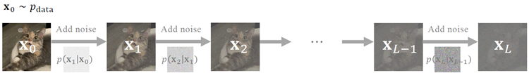
Figure 2.4: Illustration of the DDPM forward process, wherein Gaussian noise is incrementally added to corrupt a data sample into pure noise.
図2.4:DDPMの順方向プロセスを示す図。このプロセスでは、ガウスノイズが段階的に加えられ、データサンプルが徐々にノイズへと変化していく。
Let us formalize this step-by-step degradation:
この段階的な劣化プロセスを体系的に説明しましょう。
Fixed Gaussian Transitions. Each step in the forward process is governed by a fixed Gaussian transition kernel
1:
固定ガウス遷移。順方向プロセスの各ステップは、固定されたガウス遷移カーネルによって制御されます1。
1
This formulation, while potentially appearing different, is mathematically equivalent to the original DDPM transition kernel
この定式化は、見た目は異なるかもしれないが、数学的には元のDDPM遷移カーネルと等価である。
\[
p(\mathbf{x}_i|\mathbf{x}_{i−1}) := \mathcal{N}(\mathbf{x}_i;\sqrt{1 − β_i^2}\mathbf{x}_{i−1}, β_i^2\mathbf{I})
\]
Here, the process begins with \(\mathbf{x}_0\), representing a sample drawn from the real data distribution pdata . The sequence \(\{β_i\}_{i=1}^L\) denotes a pre-determined, monotonically increasing noise schedule, where each \(β_i ∈ (0 ,1)\) controls the variance of the Gaussian noise injected at step \(i\). For convenience, we dene \(α_i := \sqrt{1 − β_i^2}\). This mathematical denition is precisely equivalent to the following intuitive iterative update:
ここでは、プロセスは実データ分布 pdata からサンプリングされたサンプルである \(\mathbf{x}_0\) から始まります。数列 \(\{β_i\}_{i=1}^L\) は、事前に定められた単調増加するノイズスケジュールを表し、各 \(β_i ∈ (0 ,1)\) はステップ \(i\) で注入されるガウスノイズの分散を制御します。便宜上、\(α_i := \sqrt{1 − β_i^2}\) と定義します。この数学的な定義は、以下の直感的な反復更新式と完全に等価です。
\[
\mathbf{x}_i = α_i\mathbf{x}_{i−1} + β_i\epsilon_i
\]
where \(\epsilon_i \sim \mathcal{N}(\mathbf{0},\mathbf{I})\) are independently and identically distributed. This means at each step \(i\), we scale down the previous state \(\mathbf{x}_{i−1}\) by \(α_i\) and add a controlled amount of Gaussian noise scaled by \(β_i\).
ここで、\(\epsilon_i \sim \mathcal{N}(\mathbf{0},\mathbf{I})\) は互いに独立で同一の分布に従う確率変数である。これは、各ステップ \(i\) において、前の状態 \(\mathbf{x}_{i−1}\) を \(α_i\) 倍に縮小し、\(β_i\) 倍にスケーリングされた制御量のガウスノイズを加えることを意味する。
Perturbation Kernel and Prior Distribution. By recursively applying the transition kernels, we obtain a closed-form expression for the distribution of noisy samples at step i given the original data \(\mathbf{x}_0\):
摂動カーネルと事前分布。遷移カーネルを再帰的に適用することにより、元のデータ\(\mathbf{x}_0\)が与えられた場合のステップiにおけるノイズ付きサンプルの分布に対する閉じた形式の表現が得られます。
\[
p_i(\mathbf{x}_i|\mathbf{x}_0) = \mathcal{N}\Big(\mathbf{x}_i; \overline{α}_i\mathbf{x}_0,(1 − \overline{α}_i^2)\mathbf{I}\Big)
\]
where
\[
\overline{α}_i := \prod_{k=1}^i \sqrt{1 − β_k^2}=\prod_{k=1}^i α_k
\]
This means we can sample \(\mathbf{x}_i\) directly from \(\mathbf{x}\) as 2
これは、我々が\(\mathbf{x}_i\)を\(\mathbf{x}\)から直接サンプリングできることを意味する2。
2
For a fixed index \(t\), we will often use, both here and later on, the Gaussian perturbation form
固定されたインデックス \(t\) に対して、ここでも後でも、ガウス摂動法をよく使います。
\[
p_t(\mathbf{x}_t|\mathbf{x}_0)=\mathcal{N}(\mathbf{x}_t;α_t\mathbf{x}_0, σ_t^2 \mathbf{I})
\]
which we equivalently write as the identity in distribution
これは、分布における等式として同等に記述できる。
\[
\mathbf{x}_t \overset{d}{=}α_t\mathbf{x}_0 + σ_t\epsilon \quad
that\; is \quad Law(\mathbf{x}_t) = Law(α_t\mathbf{x}_0 + σ_t\epsilon)
\]
where \(\mathbf{x}_0 \sim p_{data}, \epsilon \sim \mathcal{N}(\mathbf{0},\mathcal{I})\) is independent of \(\mathbf{x}_0\), and \(α_t, σ_t\) are deterministic scalars. Equality “\(\overset{d}{=}\)” means the two random variables have the same probability density (i.e., law ), hence the same expectations for any test function \(\phi\):
ここで、\(\mathbf{x}_0 \sim p_{data}\) および \(\epsilon \sim \mathcal{N}(\mathbf{0},\mathcal{I})\) であり、\(\epsilon\) は \(\mathbf{x}_0\) とは独立であり、\(α_t, σ_t\) は確定的なスカラーである。等号「\(\overset{d}{=}\)」は、2つの確率変数が同じ確率密度(すなわち、同じ分布)を持つことを意味し、したがって、任意のテスト関数 \(\phi\) に対して同じ期待値を持つことを意味する。
\[
\mathbb{E}[\phi(\mathbf{x}_t)] = \mathbb{E}[\phi(α_t\mathbf{x}_0 + σ_t\epsilon)]
\]
For brevity, we will write \(\mathbf{x}_t = α_t\mathbf{x}_0 + σ_t\epsilon\), understood either as an equality in distribution or, by context, as a sample realization; this shorthand will be used throughout.
簡潔にするため、ここでは \(\mathbf{x}_t = α_t\mathbf{x}_0 + σ_t\epsilon\) と表記することにします。これは、文脈に応じて、分布における等式として、あるいは標本実現値として理解されるものとします。この略記法は以降を通して使用します。
\[
\mathbf{x}_i =\overline{α}_i\mathbf{x}_0 + \sqrt{1 − \overline{α}_i^2}\epsilon, \quad \epsilon \sim \mathcal{N}(\mathbf{0},\mathbf{I}) \tag{2.2.1}
\]
Let the noise schedule \(\{β_i\}_{i=1}~L\) be an increasing sequence, then the marginal distribution of the forward process converges as
ノイズスケジュール\(\{β_i\}_{i=1}~L\)を増加系列とすると、順方向過程の周辺分布は次のように収束する。
\[
p_L(\mathbf{x}_L|\mathbf{x}_0) −→ \mathcal{N}(\mathbf{0},\mathbf{I})\quad as\; L → ∞
\]
which motivates the choice of the prior distribution as
これは、事前分布を次のように選択する理由となる。
\[
p_{prior} := \mathcal{N}(\mathbf{0},\mathbf{I})
\]
with no reliance on data \(\mathbf{x}_0\).
データ \(\mathbf{x}_0\) に一切依存しない。
At its core, the essence of DDPMs lies in their ability to reverse the controlled degradation imposed by the forward diffusion process. Starting from pure, unstructured noise, \(\mathbf{x}_L \sim p_{prior}\) , the objective is to progressively denoise this randomness, step by step, until a coherent and meaningful data sample emerges. This reverse generation proceeds through a Markov chain, illustrated by Figure 2.5 .
DDPMの本質は、順方向拡散プロセスによって課される制御された劣化を逆転させる能力にあります。純粋で構造化されていないノイズ \(\mathbf{x}_L \sim p_{prior}\) から始めて、このランダム性を段階的にノイズ除去し、一貫性があり意味のあるデータサンプルが出現するまで続けることが目的です。この逆生成は、図2.5に示すマルコフ連鎖に沿って進行します。
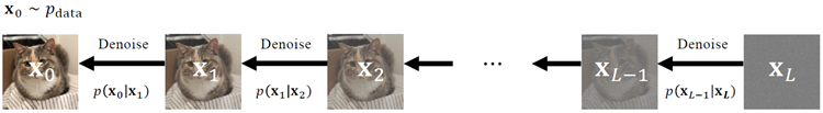
Figure 2.5: Illustration of DDPM reverse (denoising) process. Starting from noise \(\mathbf{x}_L \sim p_{prior}\), the model sequentially samples \(\mathbf{x}_{i−1} \sim p(\mathbf{x}_{i−1}|\mathbf{x}_i)\) for \(i = L,..., 1\) to obtain a newly generated data \(\mathbf{x}\). The oracle transition \(p(\mathbf{x}_{i−1}|\mathbf{x}_i)\) is unknown; thus, we aim to approximate it.
図2.5: DDPM逆(ノイズ除去)プロセスの図解。ノイズ\(\mathbf{x}_L \sim p_{prior}\)から開始し、モデルは\(i = L,..., 1\)について\(\mathbf{x}_{i−1} \sim p(\mathbf{x}_{i−1}|\mathbf{x}_i)\)を順次サンプリングし、新しく生成されたデータ\(\mathbf{x}\)を取得します。オラクル遷移\(p(\mathbf{x}_{i−1}|\mathbf{x}_i)\)は未知であるため、これを近似することを目指します。
The fundamental challenge, and the central question guiding DDPM development, then becomes:
DDPM 開発を導く基本的な課題、そして中心的な質問は次のようになります。
Question 2.2.1
Can we precisely compute, or at least effectively approximate, these reverse
transition kernels \(p(\mathbf{x}_{i−1}|\mathbf{x}_i)\), especially when considering the complex
distribution of \(\mathbf{x}_i \sim p_i(\mathbf{x}_i)\) ?
これらの逆遷移カーネル \(p(\mathbf{x}_{i−1}|\mathbf{x}_i)\) を正確に計算、あるいは少なくとも効果的に近似することは可能でしょうか?特に \(\mathbf{x}_i \sim p_i(\mathbf{x}_i)\) の複雑な分布を考慮する場合、どうなるでしょうか?
Rather than diving immediately into the mathematically intricate deriva- tion of the Evidence Lower Bound (ELBO), as the original DDPM paper does (for which a detailed discussion awaits in Section 2.2.5 ), we will instead ap- proach the training objective from a more intuitive perspective: by leveraging conditional probabilities to achieve a tractable formulation.
オリジナルのDDPM論文のように、証拠下限値(ELBO)の数学的に複雑な導出にすぐに飛び込むのではなく(詳細な議論はセクション2.2.5で待っています)、代わりに、条件付き確率を活用して扱いやすい定式化を達成することにより、より直感的な観点からトレーニング目標にアプローチします。
Overview: Modeling and Training Objective. To enable the generative process, our goal is to approximate the unknown true reverse transition kernel, \(p(\mathbf{x}_{i−1}|\mathbf{x}_i)\). We achieve this by introducing a learnable parametric model, \(p_\phi(\mathbf{x}_{i−1}|\mathbf{x}_i)\), and training it to minimize the expected KL divergence:
概要:モデリングとトレーニングの目的 生成プロセスを可能にするために、未知の真の逆遷移カーネル \(p(\mathbf{x}_{i−1}|\mathbf{x}_i)\) を近似することを目標としています。これは、学習可能なパラメトリックモデル \(p_\phi(\mathbf{x}_{i−1}|\mathbf{x}_i)\) を導入し、期待される KL ダイバージェンスを最小化するようにトレーニングすることで実現します。
\[
\mathbb{E}_{p_i(\mathbf{x}_i)}\Big[\mathcal{D}_{KL}\big(
p(\mathbf{x}_{i−1}|\mathbf{x}_i)||p_\phi(\mathbf{x}_{i−1}|\mathbf{x}_i)\big)\Big] \tag{2.2.2}
\]
However, a direct computation of the target distribution \(p(\mathbf{x}_{i−1}|\mathbf{x}_i)\) is challenging. By Bayes’ theorem, we would need to evaluate:
しかし、目標分布\(p(\mathbf{x}_{i−1}|\mathbf{x}_i)\)を直接計算するのは困難です。ベイズの定理によれば、以下を評価する必要があります。
\[
p(\mathbf{x}_{i−1}|\mathbf{x}_i) = p(\mathbf{x}_i|\mathbf{x}_{i−1})\underbrace{\frac{p_{i−1}(\mathbf{x}_{i−1})}{p_i(\mathbf{x}_i)}}_{手に負えない}
\]
The marginals \(p_i(\mathbf{x}_i)\) and \(p_{i−1}(\mathbf{x}_{i−1})\) are expectations over the unknown data distribution \(p_{data}\), given by:
周辺分布\(p_i(\mathbf{x}_i)\)と\(p_{i−1}(\mathbf{x}_{i−1})\)は未知のデータ分布\(p_{data}\)に対する期待値であり、次のように与えられる。
\[
p_i(\mathbf{x}_i) = \int p_i(\mathbf{x}_i|\mathbf{x}_0)p_{data} (\mathbf{x}_0)d \mathbf{x}_0
\]
and analogously for \(p_{i−1}(\mathbf{x}_{i−1})\). Since pdata is unknown, these integrals have no closed-form evaluation; at best they can be approximated from samples, so the exact densities are not available in practice.
\(p_{i−1}(\mathbf{x}_{i−1})\)についても同様です。pdataは未知数なので、これらの積分には閉じた形式の評価はありません。せいぜいサンプルから近似値を求めることができるので、実際には正確な密度を得ることはできません。
Overcoming Intractability with Conditioning. A central insight in DDPMs resolves this intractability: we condition the reverse transition on a clean data sample \(\mathbf{x}\). This subtle yet powerful step transforms the intractable kernel into one that is mathematically tractable:
条件付けによる扱いにくさの克服DDPMにおける中心的な洞察は、この扱いにくさを解決します。逆遷移をクリーンなデータサンプル \(\mathbf{x}\) に条件付けします。この微妙ながらも強力なステップにより、扱いにくかったカーネルが数学的に扱いやすいものへと変換されます。
\[
p(\mathbf{x}_{i−1}|\mathbf{x}_i,\mathbf{x}) =
p(\mathbf{x}_i|\mathbf{x}_{i−1})\frac{p(\mathbf{x}_{i−1}|
\mathbf{x})}{p(\mathbf{x}_i|\mathbf{x})}
\]
This tractability arises from two key properties of the forward process: its Markov property, meaning \(p(\mathbf{x}_i|\mathbf{x}_{i−1},\mathbf{x}) = p(\mathbf{x}_i|\mathbf{x}_{i−1})\), and the Gaussian nature of all involved distributions. As a result, \(p(\mathbf{x}_{i−1}|\mathbf{x}_i,\mathbf{x})\) itself is Gaussian and admits a closed-form expression (which we saw in Equation ( 2.2.4 )). Crucially, this elegant conditioning strategy allows us to derive a tractable objective that is functionally equivalent to the seemingly intractable marginal KL divergence in Equation ( 2.2.2 ).
この扱いやすさは、順方向プロセスの2つの重要な特性から生じます。マルコフ性、つまり \(p(\mathbf{x}_i|\mathbf{x}_{i−1},\mathbf{x}) = p(\mathbf{x}_i|\mathbf{x}_{i−1})\) と、関係するすべての分布のガウス分布の性質です。結果として、\(p(\mathbf{x}_{i−1}|\mathbf{x}_i,\mathbf{x})\) 自体はガウス分布であり、閉じた形式の表現が可能です(式(2.2.4)で示しました)。重要なのは、この洗練された条件付け戦略により、式(2.2.2)の一見扱いにくい周辺KLダイバージェンスと機能的に等価な扱いやすい目的関数を導出できることです。
Theorem 2.2.1: Equivalence Between Marginal and Conditional KL Minimization
定理 2.2.1: 周辺 KL 最小化と条件付き KL 最小化の同値性
The following equality holds:
次の等式が成り立ちます。
\[
\begin{align}
&\mathbb{E}_{p_i(\mathbf{x}_i)}\big[\mathcal{D}_{KL}\big(p(\mathbf{x}_{i−1}|\mathbf{x}_i)||p_\phi(\mathbf{x}_{i−1}|\mathbf{x}_i)\big)\big] \\
&= \mathbb{E}_{p_{data}(\mathbf{x})}\mathbb{E}_{p(\mathbf{x}_i|\mathbf{x})}\big[\mathcal{D}_{KL}\big(p(\mathbf{x}_{i−1}|\mathbf{x}_i,\mathbf{x})||p_\phi(\mathbf{x}_{i−1}|\mathbf{x}_i)\big)\big]+ C
\end{align}
\tag{2.2.3}
\]
where \(C\) is a constant independent of \(\phi\). Moreover, the minimizer of Equation ( 2.2.3 ) satises
ここで \(C\) は \(\phi\) に依存しない定数である。さらに、式(2.2.3)の最小値は
\[
p^∗(\mathbf{x}_{i−1}|\mathbf{x}_i) = \mathbb{E}_{p(\mathbf{x}|\mathbf{x}_i)}\big[p(\mathbf{x}_{i−1}|\mathbf{x}_i,\mathbf{x})\big] = p(\mathbf{x}_{i−1}|\mathbf{x}_i),\quad \mathbf{x}_i \sim p_i
\]
Proof for Theorem.定理の証明
The proof rewrites a KL-divergence expectation by expanding denitions, applying the chain rule of probability, and using a logarithmic identity to decompose it into the sum of an expected conditional KL divergence and a marginal KL divergence. A complete derivation is in Section D.1.1 .
証明は、KLダイバージェンスの期待値を、定義を展開し、確率の連鎖律を適用し、対数恒等式を用いて、期待値付き条件付きKLダイバージェンスと周辺KLダイバージェンスの和に分解することで書き換える。完全な導出はD.1.1節を参照。
This alternative viewpoint: conditioning to obtain a tractable objective, forms the foundation of DDPMs and reveals a profound commonality with other in‚uential diffusion models, as we will explore in Chapter 3 and Chapter 5.
この代替的な視点、すなわち扱いやすい目的を達成するための条件付けは、DDPM の基礎を形成し、第 3 章と第 5 章で検討するように、他の影響力のある普及モデルとの深い共通性を明らかにします。
It reveals a powerful equivalence: minimizing the KL divergence between marginal distributions is mathematically identical to minimizing the KL divergence between specic conditional distributions. This latter formulation is exceptionally useful because the crucial conditional distribution, p(xi−1|xi,x), possesses a convenient closed-form expression:
これは強力な同値性を示しています。周辺分布間のKLダイバージェンスを最小化することは、特定の条件付き分布間のKLダイバージェンスを最小化することと数学的に同一です。この後者の定式化は、重要な条件付き分布p(xi−1|xi,x)が便利な閉形式表現を持つため、非常に有用です。
Lemma 2.2.2: Reverse Conditional Transition Kernel
補題 2.2.2: 逆条件遷移カーネル
\(p(\mathbf{x}_{i−1}|\mathbf{x}_i,\mathbf{x})\) is Gaussian with the closed-form expression:
\(p(\mathbf{x}_{i−1}|\mathbf{x}_i,\mathbf{x})\) は閉じた形式の表現を持つガウス分布である:
\[
p(\mathbf{x}_{i−1}|\mathbf{x}_i,\mathbf{x}) = \mathcal{N}\big(\mathbf{x}_{i−1};µ(\mathbf{x}_i,\mathbf{x},i), σ^2(i)\mathbf{I}\big)
\]
where
\[
µ(\mathbf{x}_i,\mathbf{x},i) := \frac{\overline{α}_{i−1}β_i^2}{1 −\overline{α}_i^2}\mathbf{x}+\frac{(1-\overline{α}_{i-1}^2)α_i}{1-\overline{α}_i^2}\mathbf{x}_i, \quad σ^2(i) := \frac{1 −\overline{α}_{i-1}^2}{1 −\overline{α}_i^2}β_i^2 \tag{2.2.4}
\]
Later in Lemma 4.4.2 , we present a more general formula that extends beyond the DDPM noising process described in Equation ( 2.2.1 ).
補題4.4.2では、式(2.2.1)で説明したDDPMノイズ処理を超えた、より一般的な式を提示する。
Leveraging the gradient-level equivalence as in Theorem 2.2.1 and the Gaussian form of the reverse conditional \(p(\mathbf{x}_{i−1}|\mathbf{x}_i,\mathbf{x})\) as in Lemma 2.2.2 , DDPM assumes that each reverse transition \(p_\phi(\mathbf{x}_{i−1}|\mathbf{x}_i)\) is Gaussian, parameterized as
定理2.2.1の勾配レベルの同値性と補題2.2.2の逆条件式\(p(\mathbf{x}_{i−1}|\mathbf{x}_i,\mathbf{x})\)のガウス形を利用して、DDPMは各逆遷移\(p_\phi(\mathbf{x}_{i−1}|\mathbf{x}_i)\)がガウス分布であると仮定し、次のようにパラメータ化される。
\[
p_\phi(\mathbf{x}_{i−1}|\mathbf{x}_i) := \mathcal{N}
\big(\mathbf{x}_{i−1};µ_\phi(\mathbf{x}_i, i), σ^2(i)\mathbf{I}\big) \tag{2.2.5}
\]
where \(µ_\phi(·,i): \mathbb{R}^D → \mathbb{R}^D\) is a learnable mean function, and \(σ^2(i) \gt 0\) is fixed as dened in Equation (2.2.4).
ここで\(µ_\phi(·,i): \mathbb{R}^D → \mathbb{R}^D\)は学習可能な平均関数であり、\(σ^2(i) \gt 0\)は式(2.2.4)で定義されたとおりに固定される。
We denote the KL divergence, averaged over time steps \(i\) and conditioned on data \(\mathbf{x}_0 \sim p_{data}\) , to match all layers of distributions as:
すべての分布層に一致するように、時間ステップ \(i\) にわたって平均され、データ \(\mathbf{x}_0 \sim p_{data}\) に条件付けられた KL ダイバージェンスを次のように表します。
\[
\mathcal{L}_{diffusion}(\mathbf{x}_0;\phi) := \sum_{i=1}^L \mathbb{E}_{p(\mathbf{x}_i|\mathbf{x}_0)}\big[
\mathcal{D}_{KL}\big(p(\mathbf{x}_{i−1}|\mathbf{x}_i,\mathbf{x}_0)||p_\phi(\mathbf{x}_{i−1}|\mathbf{x}_i)\big)\big] \tag{2.2.6}
\]
Thanks to the Gaussian forms of both distributions and the parameterization dened in Equation (2.2.5 ), the objective admits a closed-form expression and can be simplied as:
両分布のガウス形と式(2.2.5)で定義されたパラメータ化のおかげで、目的関数は閉じた形式の表現が可能になり、次のように簡略化できる。
\[
\mathcal{L}_{diffusion}(\mathbf{x}_0;\phi) = \sum_{i=1}^L \frac{1}{2σ^2(i)}||µ_\phi(\mathbf{x}_i, i) − µ(\mathbf{x}_i,\mathbf{x}_0, i)||_2^2 + C \tag{2.2.7}
\]
where \(C\) is a constant independent of \(\phi\). Averaging over the data distribution and omitting the constant C (which does not affect the optimization), the nal DDPM training objective is
ここで、\(C\)は\(\phi\)に依存しない定数である。データ分布を平均化し、定数C(最適化には影響しない)を省略すると、最終的なDDPM訓練目標は次のようになる。
\[
\mathcal{L}_{DDPM}(\phi) := \sum_{i=1}^L \frac{1}{2σ^2(i)}\mathbb{E}_{\mathbf{x}_0}\mathbb{E}_{p(\mathbf{x}_i|\mathbf{x}_0)}\big[||µ_\phi(\mathbf{x}_i,i) − µ(\mathbf{x}_i,\mathbf{x}_0,i)||_2^2\big] \tag{2.2.8}
\]
where \(\mathbf{x}_0 \sim p_{data}\).
ここで\(\mathbf{x}_0 \sim p_{data}\)です。
\(\epsilon\)-Prediction. In typical DDPM implementations, training is not conducted directly using the original loss based on the mean prediction parameterization from Equation ( 2.2.8 ). Instead, an equivalent reparameterization, known as the \(\epsilon\)-prediction (noise prediction) formulation, is commonly adopted.
\(\epsilon\)-予測 典型的なDDPM実装では、式(2.2.8)の平均予測パラメータ化に基づく元の損失を直接用いて学習を行うことはありません。代わりに、\(\epsilon\)-予測(ノイズ予測)定式化と呼ばれる同等の再パラメータ化が一般的に採用されています。
Recall that in the DDPM forward process, a noisy sample \(\mathbf{x}_i \sim p(\mathbf{x}_i|\mathbf{x})\) at noise level \(i\) is generated by
DDPM順方向処理では、ノイズレベル\(i\)のノイズサンプル\(\mathbf{x}_i \sim p(\mathbf{x}_i|\mathbf{x})\)が次のように生成されることを思い出してください。
\[
\mathbf{x}_i = \overline{α}_i\mathbf{x}_0 + \sqrt{1 −\overline{α}_i^2}\epsilon,\quad \mathbf{x}_0 \sim p_{data},\quad \epsilon \sim \mathcal{N}(\mathbf{0},\mathbf{I}) \tag{2.2.9}
\]
Using this expression, the reverse mean \(µ(\mathbf{x}_i,\mathbf{x}_0, i)\) from Equation (2.2.4) can be rewritten as:
この式を用いると、式(2.2.4)の逆平均\(µ(\mathbf{x}_i,\mathbf{x}_0, i)\)は次のように書き直すことができる。
\[
µ(\mathbf{x}_i,\mathbf{x}_0, i) = \frac{1}{α_i}\left(\mathbf{x}_i
−\frac{1 − α_i^2}{\sqrt{1-\overline{α}_i^2}}\epsilon\right)
\]
This motivates a parameterization of the model mean \(µ_\phi\) using a neural network \(\epsilon_\phi(\mathbf{x}_i,i)\) that directly predicts the noise:
これにより、ノイズを直接予測するニューラルネットワーク\(\epsilon_\phi(\mathbf{x}_i,i)\)を使用して、モデル平均\(µ_\phi\)をパラメータ化することになります。
\[
µ_\phi(\mathbf{x}_i,i) =\frac{1}{α_i}\left(\mathbf{x}_i −\frac{1 − α_i^2}{\sqrt{1-\overline{α}_i^2}}\underbrace{\epsilon_\phi(\mathbf{x}_i,i)}_{\epsilon-予測}\right)
\]
Substituting this into the original loss leads to a squared \(ℓ_2\) error between predicted and true noise:
これを元の損失に代入すると、予測ノイズと実際のノイズの間に \(ℓ_2\) の二乗誤差が生じます。
\[
||µ_\phi(\mathbf{x}_i, i) − µ(\mathbf{x}_i,\mathbf{x}_0, i)||_2^2 ∝ ||\epsilon_\phi(\mathbf{x}_i, i) − \epsilon||_2^2
\]
up to a weighting factor depending on \(i\). Intuitively, the model acts as a “noise detective”, estimating the random noise added at each step of the forward process. Subtracting this estimate from the corrupted sample moves it closer to the clean original, and repeating this step-by-step reconstructs the data from pure noise.
\(i\) に依存する重み係数まで。直感的に言えば、このモデルは「ノイズ検出器」として機能し、順方向処理の各ステップで追加されるランダムノイズを推定します。この推定値を破損したサンプルから差し引くことで、サンプルは元のクリーンなデータに近づき、これを段階的に繰り返すことで、純粋なノイズからデータが再構築されます。
Simpli Loss with \(\epsilon\)-Prediction. In practice, this expression is further simplied by omitting the weighting term, yielding the widely used DDPM training loss:
\(\epsilon\)-予測による単純化された損失 実際には、この式は重み付け項を省略することでさらに単純化され、広く使用されている DDPM トレーニング損失が得られます。
\[
\mathcal{L}_{simple}(\phi) := \mathbb{E}_i\mathbb{E}_{\mathbf{x}\sim p_{data}(\mathbf{x})}\mathbb{E}_{\epsilon \sim \mathcal{N}(\mathbf{0},\mathbf{I})}\big[||\epsilon_\phi(\mathbf{x}_i, i) − \epsilon||_2^2\big] \tag{2.2.10}
\]
where \(\mathbf{x}_i = \overline{α}_i\mathbf{x}_0 + \sqrt{1 − \overline{α}_i^2}\epsilon\) with \(\mathbf{x}_0 \sim p_{data}\). Since the target noise has unit variance at every timestep \(t\), the \(ℓ_2\) loss in Equation (2.2.10) maintains a consistent scale across all \(t\). This prevents vanishing or exploding targets and eliminates the need for explicit loss weighting.
ここで、\(\mathbf{x}_i = \overline{α}_i\mathbf{x}_0 + \sqrt{1 − \overline{α}_i^2}\epsilon\) であり、\(\mathbf{x}_0 \sim p_{data}\) である。ターゲットノイズは各タイムステップ \(t\) で単位分散を持つため、式(2.2.10)の \(ℓ_2\) 損失はすべての \(t\) にわたって一貫したスケールを維持する。これにより、ターゲットの消失や爆発が防止され、明示的な損失の重み付けが不要になる。
Importantly, both \(\mathcal{L}_{DDPM}\) and \(\mathcal{L}_{simple}\) share the same optimal solution \(\epsilon^*\), this is because Equation (2.2.10) essentially reduces to a least-squares problem (as shown similarly in Proposition 4.2.1 or Proposition 6.3.1 ):
重要なのは、\(\mathcal{L}_{DDPM}\)と\(\mathcal{L}_{simple}\)の両方が同じ最適解\(\epsilon^*\)を共有することです。これは、式(2.2.10)が本質的に最小二乗問題に帰着するためです(命題4.2.1または命題6.3.1で同様に示されています)。
\[
\epsilon^*(\mathbf{x}_i,i)=\mathbb{E}[\epsilon|\mathbf{x}_i],\quad \mathbf{x}_i \sim p_i
\]
Intuitively, the \(\epsilon\)-prediction network \(\epsilon_\phi(\mathbf{x}_i, i)\) estimates the noise added by the forward process to produce \(\mathbf{x}_i\). At optimality, this estimate coincides with the conditional expectation of the true noise, even though \(\mathbf{x}_i\) does not uniquely
determine the original clean sample.
直感的には、\(\epsilon\)予測ネットワーク\(\epsilon_\phi(\mathbf{x}_i, i)\)は、順方向プロセスによって追加されたノイズを推定して\(\mathbf{x}_i\)を生成します。最適条件では、\(\mathbf{x}_i\)が元のクリーンサンプルを一意に決定しない場合でも、この推定値は真のノイズの条件付き期待値と一致します。
Another Equivalent Parametrization: \(\mathbf{x}\)-Prediction. Equation ( 2.2.4 ) motivates an alternative yet equivalent parameterization, known as \(\mathbf{x}\)-prediction (clean prediction), in which a neural network \(\mathbf{x}_\phi(\mathbf{x}_i, i)\) is trained to predict a clean (denoised) sample from a given noisy input \(\mathbf{x}_i \sim p_i(\mathbf{x}_i)\) at noise level \(i\). Replacing the ground-truth clean sample \(\mathbf{x}\) in the reverse mean expression with \(\mathbf{x}_\phi(\mathbf{x}_i, i)\) leads to the following model:
もう1つの同等のパラメータ化: \(\mathbf{x}\)-予測。 式 ( 2.2.4 ) は、\(\mathbf{x}\)-予測 (クリーン予測) と呼ばれる、代替でありながら同等のパラメータ化の根拠を示しています。このパラメータ化では、ニューラルネットワーク \(\mathbf{x}_\phi(\mathbf{x}_i, i)\) が、ノイズレベル \(i\) で与えられたノイズのある入力 \(\mathbf{x}_i \sim p_i(\mathbf{x}_i)\) からクリーンな (ノイズ除去された) サンプルを予測するようにトレーニングされます。逆平均式の真のクリーンサンプル \(\mathbf{x}\) を \(\mathbf{x}_\phi(\mathbf{x}_i, i)\) に置き換えると、次のモデルになります。
\[
µ_\phi(\mathbf{x}_i, i) =\frac{\overline{α}_{i−1}β_i^2}{1 − \overline{α}_i^2}\mathbf{x}_\phi(\mathbf{x}_i, i) +
\frac{(1 −\overline{α}_{i−1}^2)α_i}{1 −\overline{α}_i^2}\mathbf{x}_i
\]
Analogous to the \(\epsilon\)-prediction formulation, the training objective can be expressed as
\(\epsilon\)予測定式化と同様に、訓練目標は次のように表現できる。
\[
||µ_\phi(\mathbf{x}_i, i) − µ(\mathbf{x}_i,\mathbf{x}_0, i)||_2^2 ∝ ||\mathbf{x}_\phi(\mathbf{x}_i, i) − \mathbf{x}_0||_2^2,\quad
\mathbf{x}_0 \sim p_{data}
\]
where the model is trained to predict the original data sample \(\mathbf{x}\) from its noisy version \(\mathbf{x}_i\). This equivalence reduces the mean-matching loss in Equation (2.2.8) to
ここで、モデルは元のデータサンプル\(\mathbf{x}\)をそのノイズバージョン\(\mathbf{x}_i\)から予測するように訓練される。この同値性により、式(2.2.8)の平均マッチング損失は次のように減少する。
\[
\mathbb{E}_i\mathbb{E}_{\mathbf{x}_0 \sim p_{data}}\mathbb{E}_{\epsilon \sim \mathcal{N}(\mathbf{0},\mathbf{I})}\Big[ω_i||\mathbf{x}_\phi(\mathbf{x}_i, i) − \mathbf{x}_0||_2^2\Big]
\]
for some weighting function \(ω_i\). Since this is a least-squares problem, the optimal solution is given by (see Proposition 4.2.1 or Proposition 6.3.1 )
何らかの重み関数\(ω_i\)に対して、最小二乗問題であるため、最適解は(命題4.2.1または命題6.3.1を参照)で与えられる。
\[
\mathbf{x}^∗(\mathbf{x}_i, i) = \mathbb{E}[\mathbf{x}_0|\mathbf{x}_i], \quad \mathbf{x}_i \sim p_i \tag{2.2.11}
\]
that is, the model should predict the expected clean data given a noisy observation \(\mathbf{x}_i\) at timestep \(i\).
つまり、モデルは、タイムステップ\(i\)でのノイズの多い観測\(\mathbf{x}_i\)が与えられた場合に、期待されるクリーンなデータを予測する必要があります。
The \(\mathbf{x}\)-prediction and \(\epsilon\)-prediction parameterizations are mathematically equivalent and connected via the forward process:
\(\mathbf{x}\)予測と \(\epsilon\)予測のパラメータ化は数学的に等価であり、順方向プロセスを介して接続されています。
\[
\mathbf{x}_i = \overline{α}_i\mathbf{x}_\phi(\mathbf{x}_i, i) +
\sqrt{1−\overline{α}_i^2}\epsilon_\phi(\mathbf{x}_i, i) \tag{2.2.12}
\]
That is, one may either predict the clean sample \(\mathbf{x}_\phi(\mathbf{x}_i, i)\) or the noise \(\epsilon_\phi(\mathbf{x}_i, i)\), such that their combination reproduces \(\mathbf{x}_i\) under the forward noising process.
つまり、クリーンなサンプル \(\mathbf{x}_\phi(\mathbf{x}_i, i)\) またはノイズ \(\epsilon_\phi(\mathbf{x}_i, i)\) のいずれかを予測し、それらの組み合わせによって順方向ノイズ処理下で \(\mathbf{x}_i\) が再現されることになります。
With the reverse transitions dened as in Equation ( 2.2.5 ), this leads to the denition of the joint generative distribution in DDPM as:
逆遷移が式(2.2.5)のように定義されているので、DDPMにおける結合生成分布は次のように定義される。
\[
p_\phi(\mathbf{x}_0,\mathbf{x}_{1:L}) :=
p_\phi(\mathbf{x}_0|\mathbf{x}_1)p_\phi(\mathbf{x}_1|\mathbf{x}_2)···p_\phi(\mathbf{x}_{L−1}|\mathbf{x}_L)p_{prior}(\mathbf{x}_L)
\]
and the marginal generative model for data is given by:
データの周辺生成モデルは次のように与えられます。
\[
p_\phi(\mathbf{x}_0) := \int p_\phi(\mathbf{x}_0,\mathbf{x}_{1:L}) d\mathbf{x}_{1:L}
\]
Indeed, DDPM training via Equation ( 2.2.6 ) can be rigorously grounded in maximum likelihood estimation (Equation ( 1.1.2 )). Specically, its objective forms an ELBO, similar to those in VAEs and HVAEs from Section 2.1 , which serves as a lower bound on the log-density:
実際、式(2.2.6)によるDDPM訓練は、最尤推定(式(1.1.2))に厳密に基づいている。具体的には、その目的関数は、第2.1節の VAE や HVAE におけるものと同様のELBOを形成し、対数密度の下限値として機能する。
Theorem 2.2.3: DDPM’s ELBO
定理 2.2.3: DDPM の ELBO
\[
\begin{align}
−\log p_\phi(\mathbf{x}_0) &\leq −\mathcal{L}_{ELBO}(\mathbf{x}_0;\phi) \\
&:= \mathcal{L}_{prior}(\mathbf{x}_0) + \mathcal{L}_{recon.}(\mathbf{x}_0;\phi) + \mathcal{L}_{diffusion}(\mathbf{x}_0;\phi)
\end{align}
\tag{2.2.13}
\]
Here, each component of losses are dened as:
ここで、損失の各要素は次のように定義されます。
\[
\begin{align}
\mathcal{L}_{prior} (\mathbf{x}_0) &:= \mathcal{D}_{KL}\Big(p(\mathbf{x}_L|\mathbf{x}_0)||p_{prior}(\mathbf{x}_L)\Big) \\
\mathcal{L}_{recon.}(\mathbf{x}_0;\phi) &:= \mathbb{E}_{p(\mathbf{x}_1|\mathbf{x}_0)}[−\log p_\phi(\mathbf{x}_0|\mathbf{x}_1)] \\
\mathcal{L}_{diffusion} (\mathbf{x}_0;\phi) &=
\sum_{i=1}^L \mathbb{E}_{p(\mathbf{x}_i|\mathbf{x}_0)}\Big[\mathcal{D}_{KL}\Big(p(\mathbf{x}_{i−1}|\mathbf{x}_i,\mathbf{x}_0)||p_\phi(\mathbf{x}_{i−1}|\mathbf{x}_i)\Big)\Big]
\end{align}
\]
Proof for Theorem.
The derivation applies Jensen’s inequality, as in the HVAE/VAE ELBO (Equation ( 2.1.3 )), with further simplications. The detailed proof is de- ferred to Section D.1.2 .
導出には、HVAE/VAE ELBO(式(2.1.3))と同様に、Jensen の不等式を適用し、さらに簡略化を加える。詳細な証明はD.1.2節に譲る。
The ELBO LELBO consists of three terms:
ELBO LELBO は 3 つの用語で構成されます。
The ELBO objective \(\mathcal{L}_{ELBO}\) can also be interpreted through the lens of the Data Processing Inequality with latents \(\mathbf{z} = \mathbf{x}_{1:L}\), as illustrated in Equation ( 2.1.2 ):
ELBO目的関数\(\mathcal{L}_{ELBO}\)は、式(2.1.2)に示すように、潜在変数\(\mathbf{z} = \mathbf{x}_{1:L}\)を持つデータ処理不等式を通して解釈することもできる。
\[
\mathcal{D}_{KL}(p_{data}(\mathbf{x}_0)||p_\phi(\mathbf{x}_0)) \leq \mathcal{D}_{KL}(p(\mathbf{x}_0,
\mathbf{x}_{1:L})||p_\phi(\mathbf{x}_0,\mathbf{x}_{1:L}))
\]
where \(p(\mathbf{x}_0,\mathbf{x}_{1:L}) :=
p_{data}(\mathbf{x}_0)p(\mathbf{x}_1|\mathbf{x}_0)p(\mathbf{x}_2|\mathbf{x}_1)···p(\mathbf{x}_L|\mathbf{x}_{L−1})\) denotes the joint distribution along the forward process.
ここで、\(p(\mathbf{x}_0,\mathbf{x}_{1:L}) :=
p_{data}(\mathbf{x}_0)p(\mathbf{x}_1|\mathbf{x}_0)p(\mathbf{x}_2|\mathbf{x}_1)···p(\mathbf{x}_L|\mathbf{x}_{L−1})\)は順方向過程に沿った結合分布を表します。
Remark.
Diffusion’s variational view ts the HVAE template: the “encoder” is the
xed forward noising chain, and the latents \(\mathbf{x}_{1:T}\)
share the data dimension-
ality. Training maximizes the same ELBO. There is no learned encoder
and no per-level KL terms; instead, the objective decomposes into well-
conditioned denoising subproblems from large to small noise (coarse to fine), yielding stable optimization, and high sample quality while preserving
a coarse-to-ne hierarchy over time/noise.
拡散の変分的視点はHVAEテンプレートに基づいています。「エンコーダー」は固定された順方向ノイズチェーンであり、潜在変数\(\mathbf{x}_{1:T}\)はデータの次元を共有します。トレーニングでは同じELBOが最大化されます。学習済みのエンコーダーは存在せず、レベルごとのKL項もありません。代わりに、目的関数は、大きなノイズから小さなノイズ(粗いノイズから細かいノイズ)への適切に条件付けされたノイズ除去サブ問題に分解され、時間とノイズにわたって粗いノイズから細かいノイズへの階層構造を維持しながら、安定した最適化と高いサンプル品質を実現します。
After training the \(\epsilon\)-prediction model, \(\epsilon_{\phi^×}(\mathbf{x}_i, i)\)3, sampling is performed sequentially as illustrated in Figure 2.5 , using the parametrized transition \(p_{\phi^×}(\mathbf{x}_{i−1}|\mathbf{x}_i)\) instead.
\(\epsilon\)予測モデル\(\epsilon_{\phi^×}(\mathbf{x}_i, i)\)3をトレーニングした後、図2.5に示すように、代わりにパラメーター化された遷移\(p_{\phi^×}(\mathbf{x}_{i−1}|\mathbf{x}_i)\)を使用して、サンプリングが順次実行されます。
3
We use the symbol “×” to indicate that the model has been trained and is now frozen.
モデルがトレーニングされ、現在は固定されていることを示すために、「×」記号を使用します。
More specically, starting from a random seed \(\mathbf{x}_L \sim p_{prior} = \mathcal{N}(\mathbf{0},\mathbf{I})\), we recursively sample from \(p_{\phi^×}(\mathbf{x}_{i−1}|\mathbf{x}_i)\) following the update rule below for \(i = L, L − 1,...,1\):
より具体的には、ランダムシード \(\mathbf{x}_L \sim p_{prior} = \mathcal{N}(\mathbf{0},\mathbf{I})\) から開始し、\(i = L, L − 1,...,1\) について以下の更新規則に従って \(p_{\phi^×}(\mathbf{x}_{i−1}|\mathbf{x}_i)\) から再帰的にサンプリングします。
\[
\mathbf{x}_{i-1}←\underbrace{\frac{1}{α_i}
\Bigg(\mathbf{x}_i-\frac{1-α_i^2}{\sqrt{1-\overline{α}_i^2}}\epsilon_{\phi^×}(\mathbf{x}_i,i)\Bigg)
}_{μ_{\phi^×}(\mathbf{x}_i,i)}
+σ(i)\epsilon_i,\quad \epsilon_i \sim \mathcal{N}(\mathbf{0},\mathbf{I}) \tag{2.2.14}
\]
This “denoising” process continues until \(\mathbf{x}_0\) is obtained as the nal clean generated sample.
この「ノイズ除去」プロセスは、最終的にクリーンな生成サンプルとして \(\mathbf{x}_0\) が得られるまで続けられます。
Another Interpretation of DDPM’s Sampling. From Equation ( 2.2.12 ), the clean sample prediction corresponding to a noise estimate \(\epsilon_{\phi^×}(\mathbf{x}_i, i)\) can be expressed as
DDPMのサンプリングの別の解釈式(2.2.12)から、ノイズ推定値\(\epsilon_{\phi^×}(\mathbf{x}_i, i)\)に対応するクリーンサンプル予測は次のように表される。
\[
\mathbf{x}_{\phi^×}(\mathbf{x}_i, i) =
\frac{\mathbf{x}_i − \sqrt{1 −\overline{α}_i^2}\epsilon_{\phi^×}(\mathbf{x}_i,i)}{\overline{α}_i}
\]
Plugging this into the DDPM sampling rule in Equation ( 2.2.14 ) yields the equivalent update:
これを式(2.2.14)のDDPMサンプリング規則に代入すると、同等の更新が得られる。
\[
\mathbf{x}_{i−1} ← (\mathbf{x}_iとクリーン予測\mathbf{x}_{\phi^×}の補間) + σ(i)\epsilon_i
\]
indicating that each step is centered around the predicted clean sample, with added Gaussian noise scaled by \(σ(i)\).
これは、各ステップが予測されたクリーンなサンプルを中心に配置され、\(σ(i)\) でスケーリングされたガウスノイズが追加されていることを示しています。
This reveals that DDPM sampling can be viewed as an iterative denoising process that alternates between:
このことから、DDPM サンプリングは、次の処理を交互に実行する反復的なノイズ除去プロセスとして考えることができることがわかります。
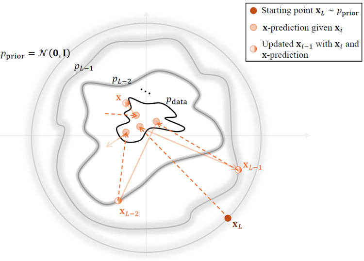
Figure 2.6: Illustration of DDPM sampling with clean prediction: estimate \(\mathbf{x}_{\phi^×}(\mathbf{x}_i, i)\) from \(\mathbf{x}_i\), then update to \(\mathbf{x}_{i−1}\).
図2.6: クリーンな予測によるDDPMサンプリングの図解: \(\mathbf{x}_i\)から\(\mathbf{x}_{\phi^×}(\mathbf{x}_i, i)\)を推定し、\(\mathbf{x}_{i−1}\)に更新します。
However, even if \(\mathbf{x}_{\phi^×}\) is trained as the optimal denoiser (i.e., the conditional expectation minimizer; see Equation ( 2.2.11 )), it can only predict the average clean sample given \(\mathbf{x}_i\). This limitation leads to blurry predictions, particularly at high noise levels, where recovering detailed structure from severely corrupted inputs becomes difficult.
しかしながら、\(\mathbf{x}_{\phi^×}\) を最適なノイズ除去器(すなわち条件付き期待値最小化器、式(2.2.11)参照)として学習させたとしても、\(\mathbf{x}_i\) が与えられた場合の平均的なクリーンサンプルしか予測できません。この制限により、特にノイズレベルが高い場合には予測結果が不鮮明になり、著しく破損した入力から詳細な構造を復元することが困難になります。
From this viewpoint, diffusion sampling typically moves from high to low noise and progressively renes an estimate of the clean signal. Early steps set the global structure, later steps add ne detail, and the sample becomes more realistic as the noise is removed.
この観点から見ると、拡散サンプリングは通常、ノイズの高いものから低いものへと移行し、クリーンな信号の推定値を徐々に改善していきます。初期のステップで全体的な構造を設定し、後のステップで詳細を追加し、ノイズが除去されるにつれてサンプルはより現実的なものになります。
Slow Sampling Speed of DDPM. DDPM (a.k.a., diffusion model) sam- pling is inherently slow 4
due to the sequential nature of its reverse process, constrained by the following factors.
DDPM のサンプリング速度が遅い DDPM(別名、拡散モデル)のサンプリングは、逆プロセスの連続的な性質により、本質的に遅くなります 4
以下の要因によって制約されます。
4
DDPM typically needs 1,000 denoising steps.
DDPM では通常、1,000 回のノイズ除去ステップが必要です。
Theorem 2.2.1 shows that an expressive \(p_\phi(\mathbf{x}_{i−1}|\mathbf{x}_i)\) can theoretically match the true reverse distribution \(p(\mathbf{x}_{i−1}|\mathbf{x}_i)\). However, in practice, \(p_\phi(\mathbf{x}_{i−1}|\mathbf{x}_i)\) is typically modeled as a Gaussian to approximate \(p(\mathbf{x}_{i−1}|\mathbf{x}_i)\), limiting its expressiveness.
定理2.2.1は、表現力のある\(p_\phi(\mathbf{x}_{i−1}|\mathbf{x}_i)\)が理論的には真の逆分布\(p(\mathbf{x}_{i−1}|\mathbf{x}_i)\)と一致することを示しています。しかし、実際には、\(p_\phi(\mathbf{x}_{i−1}|\mathbf{x}_i)\)は通常、\(p(\mathbf{x}_{i−1}|\mathbf{x}_i)\)を近似するガウス分布としてモデル化され、その表現力が制限されます。
For small forward noise scales \(β_i\), the true reverse distribution is approxi- mately Gaussian, enabling accurate approximation. Conversely, large \(β_i\) induce multimodality or strong non-Gaussianity that a single Gaussian cannot cap- ture. To maintain accuracy, DDPM employs many small \(β_i\) steps, forming a sequential chain where each step depends on the previous and requires a neural network evaluation \(\epsilon_{\phi^×}(\mathbf{x}_i, i)\). This results in \(\mathcal{O}(L)\) sequential passes, preventing parallelization and slowing generation.
前方ノイズスケール \(β_i\) が小さい場合、真の逆分布はほぼガウス分布となり、正確な近似が可能になります。一方、\(β_i\) が大きい場合、単一のガウス分布では捉えられない多峰性または強い非ガウス性が生じます。DDPM は精度を維持するために、多数の小さな \(β_i\) ステップを採用し、各ステップが前のステップに依存し、ニューラルネットワーク評価 \(\epsilon_{\phi^×}(\mathbf{x}_i, i)\) を必要とする連続チェーンを形成します。これにより、\(\mathcal{O}(L)\) 回の連続パスが発生し、並列化が妨げられ、生成速度が低下します。
Later in Chapter 4 we show a more principled interpretation of this inher- ent sampling bottleneck as a differential-equation problem, which motivates continuous-time numerical strategies for accelerating generation.
第4章の後半では、この固有のサンプリングボトルネックを微分方程式の問題としてより原理的に解釈し、生成を加速するための連続時間数値戦略を説明します。
In this chapter, we have traced the origins of diffusion models through the variational lens. We began with the Variational Autoencoder (VAE), a foun- dational generative model that learns a probabilistic mapping between data and a structured latent space via the Evidence Lower Bound (ELBO).
本章では、変分法の観点から拡散モデルの起源を辿ってきました。まず、変分オートエンコーダ(VAE)という基礎的な生成モデルから着手しました。これは、証拠下限値(ELBO)を用いて、データと構造化潜在空間との間の確率的マッピングを学習するモデルです。
We saw how Hierarchical VAEs (HVAEs) extended this idea by stacking latent layers, introducing the powerful concept of progressive, coarse-to-ne generation. However, these models face challenges with training stability and sample quality.
We then framed Denoising Diffusion Probabilistic Models (DDPMs) as a pivotal evolution within this variational framework. By fixing the encoder to a gradual noising process and learning only the reverse denoising steps, DDPMs elegantly sidestep the training instabilities of HVAEs. Crucially, we demonstrated that DDPMs are also trained by maximizing a variational bound on the log-likelihood , with a training objective that decomposes into a series of simple denoising tasks. This tractability is enabled by a powerful conditioning strategy that transforms an intractable marginal objective into a tractable conditional one, a recurring theme in diffusion models.
階層型VAE(HVAE)が潜在層を積み重ねることでこの考え方を拡張し、段階的に粗から中程度のレベルへと生成するという強力な概念を導入したことを我々は見てきました。しかし、これらのモデルは訓練の安定性とサンプル品質の点で課題を抱えています。
そこで我々は、この変分フレームワークにおける極めて重要な進化として、ノイズ除去拡散確率モデル(DDPM)を位置づけました。エンコーダーを段階的なノイズ除去プロセスに固定し、逆ノイズ除去ステップのみを学習することで、DDPMはHVAEの訓練における不安定性を巧みに回避します。重要な点として、DDPMは対数尤度の変分限界を最大化することでも訓練され、訓練目標は一連の単純なノイズ除去タスクに分解できることを示しました。この扱いやすさは、扱いにくい周辺目標を扱いやすい条件付き目標に変換する強力な条件付け戦略によって実現されており、これは拡散モデルにおいて繰り返し登場するテーマです。
While this variational framework provides a complete and powerful founda- tion for DDPMs, it is not the only way to understand them. An alternative and equally fundamental perspective emerges from the principles of energy-based modeling. In the next chapter, we will explore this score-based perspective:
この変分枠組みはDDPMの完全かつ強力な基盤を提供しますが、DDPMを理解する唯一の方法ではありません。エネルギーベースモデリングの原理から、代替的かつ同様に基本的な視点が生まれます。次の章では、このスコアベースの視点について考察します。
This alternative viewpoint will not only offer new insights but also serve as another cornerstone for the unied, continuous-time framework of diffusion models to be developed later.
この代替的な視点は、新たな洞察を提供するだけでなく、後で開発される普及モデルの統一された連続時間フレームワークのもう 1 つの基礎としても役立ちます。