What I cannot create, I do not understand.
作れないものは、理解できない。
Richard P. Feynman
Deep generative models (DGMs) are neural networks that learn a proba- bility distribution over high-dimensional data (e.g., images, text, audio) so they can generate new examples that resemble the dataset. We denote the model distribution by \(p_\phi\) and the data distribution by pdata . Given a nite dataset, we fit \(\phi\) by minimizing a loss that measures how far \(p_\phi\) is from \(p_{data}\) . After training, generation amounts to running the model’s sampling procedure to draw \(\mathbf{x} \sim p_\phi\) (the density \(p_\phi(\mathbf{x})\) may or may not be directly computable, depending on the model class). Model quality is judged by how well generated samples and their summary statistics match those of pdata , together with task-specic or perceptual metrics.
深層生成モデル(DGM)は、高次元データ(画像、テキスト、音声など)の確率分布を学習するニューラルネットワークであり、データセットに類似した新しいサンプルを生成することができます。モデルの分布を \(p_\phi\)、データ分布を \(p_{data}\) と表記します。有限のデータセットが与えられた場合、\(p_\phi\) と \(p_{data}\) の間の距離を測る損失関数を最小化することで、パラメータ \(\phi\) を学習します。学習後、生成はモデルのサンプリング手順を実行して \(\mathbf{x} \sim p_\phi\) をサンプリングすることによって行われます(モデルの種類によっては、密度関数 \(p_\phi(\mathbf{x})\) が直接計算可能である場合とそうでない場合があります)。モデルの品質は、生成されたサンプルとその要約統計量が \(p_{data}\) のものとどれだけ一致するか、およびタスク固有の指標や知覚的な指標によって評価されます。
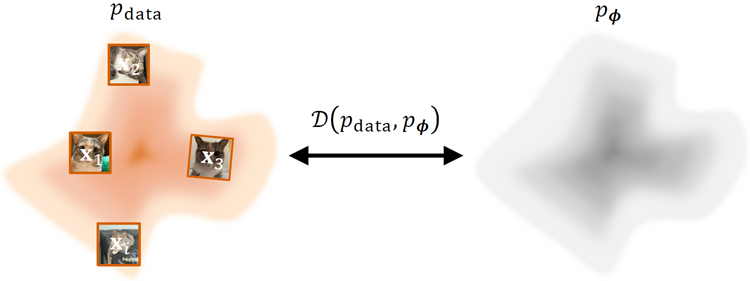
Figure 1.1: Illustration of the target in DGM. Training a DGM is essentially minimizing the discrepancy between the model distribution \(p_\phi\) and the unknown data distribution \(p_{data}\). Since \(p_{data}\) is not directly accessible, this discrepancy must be estimated efficiently using a e set of independent and identically distributed (i.i.d.) samples, \(\mathbf{x}_i\), drawn from it.
図1.1:DGMにおける学習目標の図解。DGMの学習とは、本質的にモデル分布 \(p_\phi\) と未知のデータ分布 \(p_{data}\) との間の乖離を最小化することです。\(p_{data}\) は直接アクセスできないため、この乖離は、\(p_{data}\) から抽出された独立同分布(i.i.d.)のサンプル集合 \(\mathbf{x}_i\) を用いて効率的に推定する必要があります。
This chapter builds the mathematical and conceptual foundations behind these ideas. We formalize the problem in Section 1.1 , present representa- tive model classes in Section 1.2 , and summarize a practical taxonomy in Section 1.3 .
本章では、これらのアイデアの背後にある数学的および概念的な基礎を構築します。1.1節では問題を定式化し、1.2節では代表的なモデルクラスを提示し、1.3節では実用的な分類体系をまとめます。
DGMs take as input a large collection of real-world examples (e.g., images, text) drawn from an unknown and complex distribution \(p_{data}\) and output a trained neural network that parameterizes an approximate distribution \(p_\phi\). Their goals are twofold:
DGM(深層生成モデル)は、未知の複雑な分布 \(p_{data}\) から抽出された現実世界の多数の事例(画像、テキストなど)をインプットとして受け取り、近似分布 \(p_\phi\) をパラメータ化する訓練済みニューラルネットワークを出力します。その目的は以下の2つです。
This section presents the fundamental concepts and motivations behind DGMs, preparing for a detailed exploration of their mathematical framework and practical applications.
このセクションでは、DGMの背後にある基本的な概念と動機について説明し、その数学的な枠組みと実際的な応用についての詳細な考察に備えます。
We assume access to a nite set of samples drawn independently and identically distributed (i.i.d.) from an underlying, complex data distribution \(p_{data}(x)\)1.
我々は、根底にある複雑なデータ分布 \(p_{data}(x)\)1 から独立同分布(i.i.d.)に従って抽出された有限個のサンプルにアクセスできると仮定する。
1 This is a common assumption in machine learning. For simplicity, we use the symbol \(p\) to represent either a probability distribution or its probability density/mass function,
depending on the context.
これは機械学習における一般的な前提です。簡潔にするため、文脈に応じて確率分布またはその確率密度関数/確率質量関数のいずれかを表す記号として \(p\) を使用します。
Goal of DGM. The primary goal of DGM is to learn a tractable probability distribution from a nite dataset. These data points are observations assumed to be sampled from an unknown and complex true distribution \(p_{data} (\mathbf{x})\). Since the form of \(p_{data}(\mathbf{x})\) is unknown, we cannot draw new samples from it directly. The core challenge is therefore to create a model that approximates this distribution well enough to enable the generation of new, realistic samples.
DGMの目標 DGMの主な目標は、有限のデータセットから扱いやすい確率分布を学習することです。これらのデータ点は、未知の複雑な真の分布 \(p_{data}(\mathbf{x})\) からサンプリングされた観測値であると仮定されます。\(p_{data}(\mathbf{x})\) の形式は不明であるため、そこから直接新しいサンプルを生成することはできません。したがって、中心的な課題は、この分布を十分に近似し、現実的な新しいサンプルを生成できるモデルを構築することです。
To this end, a DGM uses a deep neural network to parameterize a model distribution \(p_\phi(x)\), where \(\phi\) represents the network’s trainable parameters. The training objective is to nd the optimal parameters \(\phi^*\) that minimize the divergence between the model distribution \(p_\phi(\mathbf{x})\) and the true data distribution \(p_{data} (\mathbf{x})\). Conceptually,
この目的のため、DGMはディープニューラルネットワークを用いてモデル分布 \(p_\phi(x)\) をパラメータ化する。ここで\(\phi\)はネットワークの学習可能なパラメータを表す。学習の目的は、モデル分布 \(p_\phi(\mathbf{x})\) と真のデータ分布 \(p_{data} (\mathbf{x})\) の乖離を最小化する最適なパラメータ \(\phi^*\) を見つけることである。概念的には、
\[
p_{\phi^∗}(\mathbf{x}) \approx p_{data}(\mathbf{x})
\]
When the statistical model \(p_{\phi^*}(\mathbf{x})\) closely approximates the data distribution \(p_{data}(\mathbf{x})\), it can serve as a proxy for generating new samples and evaluating probability values. This model\(p_\phi(\mathbf{x})\) is commonly referred to as a generative model .
統計モデル \(p_{\phi^*}(\mathbf{x})\) がデータ分布 \(p_{data}(\mathbf{x})\) を高い精度で近似する場合、このモデルは新しいサンプルを生成したり、確率値を評価したりするための代替手段として利用できます。このようなモデル \(p_\phi(\mathbf{x})\) は一般的に生成モデルと呼ばれます。
Capability of DGM. Once a proxy of the data distribution, \(p_\phi(\mathbf{x})\), is available, we can generate an arbitrary number of new data points using sampling methods such as Monte Carlo sampling from \(p_\phi(\mathbf{x})\). Additionally, we can compute the probability (or likelihood) of any given data sample \(\mathbf{x}^\prime\) by evaluating \(p_\phi(\mathbf{x}^\prime)\).
DGMの能力 データ分布の近似モデルである \(p_\phi(\mathbf{x})\) が得られれば、モンテカルロサンプリングなどのサンプリング手法を用いて、 \(p_\phi(\mathbf{x})\) から任意の数の新しいデータ点を生成できます。さらに、任意のデータサンプル \(\mathbf{x}^\prime\) の確率(または尤度)は、\(p_\phi(\mathbf{x}^\prime)\) を評価することで計算できます。
Training of DGM. We learn parameters \(\phi\) of a model family \(\{p_\phi\}\) by minimizing a discrepancy \(\mathcal{D}(p_{data} , p_\phi)\):
DGMの学習 我々は、モデルファミリー \(\{p_\phi\}\) のパラメータ \(\phi\) を、不一致度 \(\mathcal{D}(p_{data} , p_\phi)\) を最小化することによって学習します。
\[
\phi^∗ ∈ arg \min\limits_{\phi}\mathcal{D}(p_{data} ,p_{\phi}) \tag{1.1.1}
\]
Because \(p_{data}\) is unknown, a practical choice of \(\mathcal{D}\) must admit efficient estimation from i.i.d. samples from \(p_{data}\) . With sufficient capacity, \(p_{\phi^*}\) can closely approximate \(p_{data}\) .
\(p_{data}\) が未知であるため、実際的な選択肢として、集合\(\mathcal{D}\) は \(p_{data}\) からの独立同分布サンプルから効率的に推定できるものでなければならない。十分な表現力があれば、\(p_{\phi^*}\)は \(p_{data}\) を高い精度で近似することができる。
Forward KL and Maximum Likelihood Estimation (MLE). choice is the (forward) Kullback–Leibler divergence
2
順方向KLダイバージェンスと最尤推定(MLE) 選択肢は(順方向)カルバック・ライブラー情報量2です。
2All integrals are in the Lebesgue sense and reduce to sums under counting measures.
すべての積分はルベーグ積分の意味であり、計数測度のもとでは和に帰着する。
\[
\begin{align}
\mathcal{D}_{KL}(p_{data}||p_\phi) &:= \int p_{data}(\mathbf{x})\log\frac{p_{data}(\mathbf{x})}{p_\phi(\mathbf{x})}d\mathbf{x} \\
\\
&=\mathbb{E}_{\mathbf{x}\sim p_{data}}[\log p_{data}(\mathbf{x})-\log p_\phi(\mathbf{x})]
\end{align}
\]
which is asymmetric, i.e.,
それは非対称である。つまり、
\[
\mathcal{D}_{KL} (p_{data}||p_\phi) \neq \mathcal{D}_{KL}(p_\phi||p_{data})
\]
Importantly, minimizing \(\mathcal{D}_{KL}(p_{data}||p_\phi)\) encourages mode covering : if there exists a set of positive measure \(A\) with \(p_{data}(A) \gt 0\) but \(p_\phi(x) = 0\) for \(x ∈ A\), then the integrand contains \(\log(p_{data}(\mathbf{x})/0 = +∞\) on \(A\), so \(\mathcal{D}_{KL} = +∞\). Thus minimizing forward KL forces the model to assign probability wherever the data has support.
重要な点として、\( \mathcal{D}_{KL}(p_{data}||p_\phi) \) を最小化することは、モードカバレッジを促進します。もし、正の測度を持つ集合 \(A\) が存在し、\(p_{data}(A) > 0\) であるにもかかわらず、\(x \in A\) に対して \(p_\phi(x) = 0\) である場合、積分項は \(A\) 上で \( \log(p_{data}(\mathbf{x})/0) = +\infty \) となるため、\( \mathcal{D}_{KL} = +\infty \) となります。したがって、順方向KLダイバージェンスを最小化することで、モデルはデータがサポートを持つすべての領域に確率を割り当てるように促されます。
Although the data density \(p_{data}(\mathbf{x})\) cannot be evaluated explicitly, the forward KL divergence can be decomposed as
データ密度\(p_{data}(\mathbf{x})\)は明示的に評価できないが、順方向KLダイバージェンスは次のように分解できる。
\[
\begin{align}
\mathcal{D}_{KL}(p_{data}||p_\phi) &=\mathbb{E}_{\mathbf{x}\sim p_{data}}\left[\log\frac{p_{data}(\mathbf{x})}{p_\phi(\mathbf{x})}\right] \\
\\
&=-\mathbb{E}_{\mathbf{x}\sim p_{data}}[\log p_\phi(\mathbf{x})]+\mathcal{H}(p_{data})
\end{align}
\]
where \(\mathcal{H}(p_{data}) := -\mathbb{E}_{\mathbf{x}\sim p_{data}}[\log p_{data}(\mathbf{x})]\) is the entropy of the data distri- bution, which is constant with respect to \(\phi\). This observation implies the following equivalence:
ここで、\(\mathcal{H}(p_{data}) := -\mathbb{E}_{x\sim p_{data}}[\log p_{data}(\mathbf{x})]\) はデータ分布のエントロピーであり、\(\phi\) に関して定数である。この観察は、以下の等価性を示唆している。
Lemma 1.1.1: Minimizing KL ⇔ MLE
補題1.1.1:KLダイバージェンスの最小化 ⇔ 最尤推定
\[ \min\limits_\phi \mathcal{D}_{KL}(p_{data}||p_\phi) \Longleftrightarrow \mathbb{E}_{\mathbf{x}\sim p_{data }}[\log p_\phi(\mathbf{x})] \tag{1.1.2} \]
In other words, minimizing the forward KL divergence is equivalent to performing MLE.
言い換えれば、順方向KLダイバージェンスを最小化することは、最尤推定(MLE)を行うことと同等である。
In practice we replace the population expectation by its Monte Carlo estimate from i.i.d. samples \(\{\mathbf{x}^{(i)}\}_{i=1}^N \sim p_{data}\) , yielding the empirical MLE objective
実際には、母集団期待値を、独立同分布に従うサンプル \(\{\mathbf{x}^{(i)}\}_{i=1}^N \sim p_{data}\) から得られたモンテカルロ推定値で置き換えることで、経験的な最尤推定の目的関数が得られる。
\[
\hat{\mathcal{L}}_{MLE}(\phi):=-\frac{1}{N}\sum_{i=1}^N \log p_\phi\left(\mathbf{x}^{(i)}\right)
\]
optimized via stochastic gradients over minibatches; no evaluation of \(p_{data}(\mathbf{x})\) is required.
ミニバッチを用いた確率的勾配法によって最適化されるため、\(p_{data}(\mathbf{x})\) の評価は不要である。
Fisher Divergence. The Fisher divergence is another important concept for (score-based) diffusion modeling (see Chapter 3). For two distributions \(p\) and \(q\), it is dened as
フィッシャーダイバージェンス フィッシャーダイバージェンスは、(スコアベースの)拡散モデル(第3章参照)におけるもう一つの重要な概念である。2つの分布\(p\)と\(q\)について、以下のように定義される。
\[
\mathcal{D}_F(p||q) := \mathbb{E}_{\mathbf{x}\sim p}\left[||\nabla_\mathbf{x} \log p(\mathbf{x})-\nabla_\mathbf{x} \log q(\mathbf{x})||_2^2\right] \tag{1.1.3}
\]
It measures the discrepancy between the score functions \(∇_\mathbf{x} \log p(\mathbf{x})\) and \(∇_\mathbf{x} \log q(\mathbf{x})\), which are vector elds pointing toward regions of higher probability. In short, \(\mathcal{D}_F(p||q) \geq 0\) with equality if and only if \(p = q\) almost everywhere.
これは、確率の高い領域を指すベクトル場であるスコア関数 \(∇_\mathbf{x} \log p(\mathbf{x})\) と \(∇_\mathbf{x} \log q(\mathbf{x})\) との間の差異を測定するものです。要するに、\(\mathcal{D}_F(p||q) \geq 0\) であり、等号は \(p = q\) がほとんど至るところで成り立つ場合にのみ成立します。
It is invariant to normalization constants, since scores depend only on gradients of log-densities, and it forms the basis of score matching (Equations ( 3.1.3 ) and ( 3.2.1 )): a method that learns the gradient of the log-density for generation (score-based models). In this setting, the data distribution \(p = p_{data}\ serves as the target, while the model \)q = p_\phi\) is trained to align its score eld with that of the data.
これは正規化定数に対して不変です。なぜなら、スコアは対数密度の勾配のみに依存するからです。そして、これはスコアマッチング(式(3.1.3)および(3.2.1))の基礎となります。スコアマッチングは、生成のための対数密度の勾配を学習する手法です(スコアベースモデル)。この設定では、データ分布 \(p = p_{data}\) が目標となり、モデル \(q = p_\phi\) はそのスコア場をデータのスコア場に一致させるように学習されます。
Beyond KL. Although the KL divergence is the most widely used measure of difference between probability distributions, it is not the only one. Different divergences capture different geometric or statistical notions of discrepancy, which in turn affect the optimization dynamics of learning algorithms. A broad family is the \(f\)-divergences (Csiszár, 1963):
KLダイバージェンスを超えて。 KLダイバージェンスは確率分布間の差異を測る最も広く用いられている指標ですが、唯一のものではありません。様々なダイバージェンスは、それぞれ異なる幾何学的または統計的な差異の概念を捉えており、それが学習アルゴリズムの最適化ダイナミクスに影響を与えます。その中でも幅広いファミリーを形成するのがf-ダイバージェンスです(Csiszár、1963)。
\[
\mathcal{D}_f(p||q) = \int q(\mathbf{x})f\left(\frac{p(\mathbf{x})}{q(\mathbf{x})}\right)d\mathbf{x}, \quad f(1)=0 \tag{1.1.4}
\]
where \(f : \mathbb{R}_+ → \mathbb{R}\) is a convex function. By changing \(f\), we obtain many well-known divergences:
ここで、\(f : \mathbb{R}_+ → \mathbb{R}\) は凸関数である。関数 \(f\) を変更することで、多くのよく知られたダイバージェンスが得られる。
\[
\begin{array}{l l l i}
f(u) = u\log u & ⇒ & \mathcal{D}_f= \mathcal{D}_{KL}(p||q) & (forward KL)\\
\\
f(u) =\frac{1}{2}\left[u\log u-(u+1)\log \frac{1+u}{2}\right] & ⇒ & \mathcal{D}_f= \mathcal{D}_{JS} (p||q) & (Jensen–Shannon) \\
\\
f(u) = \frac{1}{2}[u-1] & ⇒ & \mathcal{D}_f= \mathcal{D}_{TV}(p, q) & (total variation)\\
\end{array}
\]
For clarity, the explicit forms are
明確にするために、明示的な形式は
\[
\mathcal{D}_{JS}(p||q) = \frac{1}{2}\mathcal{D}_{KL}(p||\frac{1}{2}(p + q)) + \frac{1}{2}\mathcal{D}_{KL}(q||\frac{1}{2}(p + q))
\]
and
\[
\mathcal{D}_{TV}(p,q) = \frac{1}{2}\int_{\mathbb{R}^D} |p − q|dx = \sup\limits_{A\subset \mathbb{R}^D} |p(A) − q(A)|
\]
Intuitively, the JS divergence provides a smooth and symmetric measure that balances both distributions and avoids the unbounded penalties of KL (we will later see that it helps interpret the Generative Adversarial Network (GAN) framework), while the total variation distance captures the largest possible probability difference between the two.
直感的に言えば、JSダイバージェンスは、両方の分布のバランスを取り、KLダイバージェンスのような無限大になるペナルティを回避する、滑らかで対称的な尺度を提供する(後述するように、これは敵対的生成ネットワーク(GAN)フレームワークの解釈に役立つ)一方、全変動距離は、2つの分布間の可能な限り最大の確率差を捉える。
A different viewpoint comes from optimal transport (see Chapter 7), whose representative is the Wasserstein distance (see . It measures the minimal cost of moving probability mass from one distribution to another. Unlike \(f\)-divergences, which compare density ratios, Wasserstein distances depend on the geometry of the sample space and remain meaningful even when the supports of \(p\) and \(q\) do not overlap.
異なる観点は最適輸送(第 7 章を参照)から来ており、その代表例としてワッサーシュタイン距離(を参照)が挙げられます。これは、確率質量を 1 つの分布から別の分布に移動する際の最小コストを測定します。密度比を比較する \(f\) ダイバージェンスとは異なり、ワッサーシュタイン距離は標本空間の形状に依存し、\(p\) と \(q\) のサポートが重ならなくても意味を持ちます。
Each divergence embodies a different notion of closeness between distri- butions and thus induces distinct learning behavior. We will revisit these divergences when they arise naturally in the context of generative modeling
throughout this monograph.
それぞれのダイバージェンスは、分布間の近さという異なる概念を体現しており、それによって異なる学習行動を引き起こします。これらのダイバージェンスは、生成モデリングの文脈において自然に生じる際に、本モノグラフ全体を通して再び取り上げます。
To model a complex data distribution, we can parameterize the probability density function \(p_{data}\) using a neural network with parameters \(\phi\), creating a model we denote as \(p_\phi\). For \(p_\phi\) to be a valid probability density function, it must satisfy two fundamental properties:
複雑なデータ分布をモデル化するために、確率密度関数 \(p_{data}\) をパラメータ\(\phi\)を持つニューラルネットワークを用いてパラメータ化し、\(p_\phi\)と表記するモデルを作成します。\(p_\phi\)が有効な確率密度関数であるためには、以下の2つの基本的な特性を満たす必要があります。
A network can naturally produce a real scalar \(E_\phi(\mathbf{x}) ∈ \mathbb{R}\) for input \(\mathbf{x}\). To interpret this output as a valid density, it must be transformed to satisfy conditions (i) and (ii). A practical alternative is to view \(E_\phi: \mathbb{R}^D → \mathbb{R}\) as dening an unnormalized density and then enforce these properties explicitly.
ネットワークは、入力 \(\mathbf{x}\) に対して、実スカラー \(E_\phi(\mathbf{x}) ∈ \mathbb{R}\) を自然に生成できます。この出力を有効な密度として解釈するには、条件 (i) と (ii) を満たすように変換する必要があります。実用的な代替案としては、\(E_\phi: \mathbb{R}^D → \mathbb{R}\) を非正規化密度として定義するものと見なし、これらの特性を明示的に適用する方法があります。
Step 1: Ensuring Non-Negativity. We can guarantee that our model’s output is always non-negative by applying a positive function to the raw output of the neural network \(E_\phi(\mathbf{x})\), such as \(|E_\phi(\mathbf{x})|, E_\phi^2(\mathbf{x})\). A standard and convenient choice is the exponential function. This gives us an unnormalized density, \(\tilde{p}_\phi(\mathbf{x})\), that is guaranteed to be positive:
ステップ1:非負性の保証 ニューラルネットワークの生の出力 \(E_\phi(\mathbf{x})\) に正の関数(例えば \(|E_\phi(\mathbf{x})|, E_\phi^2(\mathbf{x})\))を適用することで、モデルの出力が常に非負であることを保証できます。標準的で便利な選択肢は指数関数です。これにより、正であることが保証された非正規化密度 \(\tilde{p}_\phi(\mathbf{x})\) が得られます。
\[
\tilde{p}_\phi(\mathbf{x}) = exp(E_\phi(\mathbf{x}))
\]
Step 2: Enforcing Normalization. The function \(\tilde{p}_\phi(\mathbf{x})\) is positive but does
not integrate to one. To create a valid probability density, we must divide it by its integral over the entire space. This leads to the nal form of our model:
ステップ2:正規化の強制 関数 \(\tilde{p}_\phi(\mathbf{x})\) は正ですが、積分すると1になりません。有効な確率密度を得るには、これを空間全体にわたる積分で割る必要があります。これにより、モデルの最終的な形が得られます。
\[
p_\phi(\mathbf{x}) = \frac{\tilde{p}_\phi(\mathbf{x})}{\int \tilde{p}_\phi(\mathbf{x}^\prime)dx^\prime}=\frac{exp(E_\phi(\mathbf{x}))}{\int exp(E_\phi(\mathbf{x}^\prime))d\mathbf{x}^\prime}
\]
The denominator in this expression is known as the normalizing constant or partition function , denoted by \(Z(\phi)\):
この式の分母は正規化定数または分割関数と呼ばれ、\(Z(\phi)\) と表記されます。
\[
Z(\phi) := \int exp(E_\phi(\mathbf{x}^\prime)) d\mathbf{x}^\prime.
\]
While this procedure provides a valid construction for \(p_\phi(\mathbf{x})\), it introduces a major computational challenge. For most high-dimensional problems, the integral required to compute the normalizing constant \(Z(\phi)\) is intractable. This intractability is a central problem that motivates the development of many different families of deep generative models.
この手順は \(p_\phi(\mathbf{x})\) の有効な構成を提供しますが、計算上の大きな課題をもたらします。ほとんどの高次元問題において、正規化定数 \(Z(\phi)\) を計算するために必要な積分は計算不可能です。この計算困難性は、様々な深層生成モデルの開発の動機となる中心的な問題です。
In the following sections, we introduce several prominent approaches of DGM. Each is designed to circumvent or reduce the computational cost of evaluating this normalizing constant.
以下のセクションでは、DGMの主要なアプローチをいくつか紹介します。それぞれのアプローチは、この正規化定数の評価にかかる計算コストを回避または削減するように設計されています。
A central challenge in generative modeling is to learn expressive probabilistic models that can capture the rich and complex structure of high-dimensional data. Over the years, various modeling strategies have been developed, each making different trade-offs between tractability, expressiveness, and training efficiency. In this section, we explore some of the most in‚uential strategies that have shaped the eld, accompanied by a comparison of their computation graphs in Figure 1.2.
生成モデリングにおける中心的な課題は、高次元データの豊かで複雑な構造を捉えることができる表現力豊かな確率モデルを学習することです。長年にわたり、様々なモデリング戦略が開発されてきましたが、それぞれが扱いやすさ、表現力、学習効率の間で異なるトレードオフを行っています。本セクションでは、この分野を形作ってきた最も影響力のある戦略のいくつかを考察し、図1.2にそれらの計算グラフの比較を示します。
Energy-Based Models (EBMs). EBMs (Ackley et al. , 1985; LeCun et al. , 2006) dene a probability distribution through an energy function \(E_\phi(\mathbf{x})\) that assigns lower energy to more probable data points. The probability of a data point is dened as:
エネルギーベースモデル(EBM)EBM(Ackley et al. , 1985; LeCun et al. , 2006)は、より確率の高いデータ点に低いエネルギーを割り当てるエネルギー関数 \(E_\phi(\mathbf{x})\) を通じて確率分布を定義します。データ点の確率は以下のように定義されます。
\[
p_\phi(\mathbf{x}):=\frac{1}{Z(\phi)}exp( −E_φ(\mathbf{x}))
\]
where
\[
Z(\phi) = \int exp( −E_\phi(\mathbf{x})) d\mathbf{x}
\]
is the partition function. Training EBMs typically involves maximizing the log-likelihood of the data. However, this requires techniques to address the computational challenges arising from the intractability of the partition func- tion. In the following chapter, we will explore how Diffusion Models offer an alternative by generating data from the gradient of the log density , which does not depend on the normalizing constant, thereby circumventing the need for partition function computation.
は分配関数です。EBMの学習では、通常、データの対数尤度を最大化します。しかし、これには、分配関数の扱いにくさから生じる計算上の課題に対処する技術が必要です。次の章では、拡散モデルが、正規化定数に依存しない対数密度の勾配からデータを生成することで、分配関数の計算を回避し、代替手段を提供する方法を探ります。
Autoregressive Models. Deep autoregressive (AR) models (Frey et al. , 1995; Larochelle and Murray, 2011; Uria et al. , 2016) factorize the joint data distribution pdata into a product of conditional probabilities using the chain rule of probability:
自己回帰モデル。深層自己回帰(AR)モデル(Frey et al. , 1995; Larochelle and Murray, 2011; Uria et al. , 2016)は、確率の連鎖律を用いて、結合データ分布pdataを条件付き確率の積に因数分解します。
\[
p_{data}(\mathbf{x}) = \prod_{i=1}^D p_\phi(x_i|\mathbf{x}_{\lt i})
\]
where \(\mathbf{x} = (x_1,..., x_D)\) and \(\mathbf{x}_{\lt i} = (x_1,..., x_{i−1})\).
ここで \(\mathbf{x} = (x_1,..., x_D)\) かつ \(\mathbf{x}_{\lt i} = (x_1,..., x_{i−1})\) である。
Each conditional \(p_\phi(x_i|\mathbf{x}_{\lt i})\) is parameterized by a neural network, such as a Transformer, allowing ‚exible modeling of complex dependencies. Because each term is normalized by design (e.g., via softmax for discrete or parameterized Gaussian for continuous variables), global normalization is trivial.
各条件付き \(p_\phi(x_i|\mathbf{x}_{\lt i})\) は、Transformerなどのニューラルネットワークによってパラメータ化され、複雑な依存関係を柔軟にモデル化できます。各項は設計上正規化されているため(例えば、離散変数の場合はソフトマックス、連続変数の場合はパラメータ化されたガウス分布)、グローバルな正規化は簡単です。
Training proceeds by maximizing the exact likelihood, or equivalently minimizing the negative log-likelihood,
訓練は正確な尤度を最大化すること、または負の対数尤度を最小化することで進行する。
While AR models achieve strong density estimation and exact likelihoods, their sequential nature limits sampling speed and may restrict ‚exibility due to xed ordering. Nevertheless, they remain a foundational class of likelihood- based generative models and key approaches in modern research.
AR モデルは強力な密度推定と正確な尤度を実現しますが、その逐次的な性質によりサンプリング速度が制限され、固定された順序付けにより柔軟性が制限される可能性があります。それでもなお、AR モデルは尤度に基づく生成モデルの基礎クラスであり、現代研究における重要なアプローチとなっています。
Variational Autoencoders (VAEs). VAEs (Kingma and Welling, 2013) extend classical autoencoders by introducing latent variables \(\mathbf{z}\) that capture hidden structure in the data \(x\). Instead of directly learning a mapping between \(\mathbf{x}\) and \(\mathbf{z}\), VAEs adopt a probabilistic view: they learn both an encoder , \(q_θ(\mathbf{z}|\mathbf{x})\), which approximates the unknown distribution of latent variables given the data, and a decoder , \(p_\phi(\mathbf{x}|\mathbf{z})\), which reconstructs data from these latent vari- ables. To make training feasible, VAEs maximize a tractable surrogate to the true log-likelihood, called the Evidence Lower Bound (ELBO):
変分オートエンコーダー (VAEs). VAE (Kingma and Welling, 2013) は、データ \(\mathbf{x}\) の隠れた構造を捉える潜在変数 \(\mathbf{z}\) を導入することで、従来のオートエンコーダーを拡張します。\(\mathbf{x}\) と \(\mathbf{z}\) 間のマッピングを直接学習する代わりに、VAE は確率的な視点を採用します。つまり、データが与えられた場合に潜在変数の未知の分布を近似するエンコーダー \(q_θ(\mathbf{z}|\mathbf{x})\) と、これらの潜在変数からデータを再構成するデコーダー \(p_\phi(\mathbf{x}|\mathbf{z})\) の両方を学習します。トレーニングを実行可能にするために、VAE は、証拠下限値 (ELBO) と呼ばれる、真の対数尤度の扱いやすい代理値を最大化します。
\[
\mathcal{L}_{ELBO}(θ,\phi;\mathbf{x}) = \mathbb{E}_{qθ(\mathbf{z}|\mathbf{x})}[\log p_\phi(\mathbf{x}|\mathbf{z})] − \mathcal{D}_{KL}(q_θ(\mathbf{z}|\mathbf{x})||p_{prior}(\mathbf{z}))
\]
.
Here, the rst term encourages accurate reconstruction of the data, while the second regularizes the latent variables by keeping them close to a simple prior distribution \(p_{prior}(\mathbf{z})\) (often Gaussian).
ここで、最初の項はデータの正確な再構築を促進し、2 番目の項は潜在変数を単純な事前分布 \(p_{prior}(\mathbf{z})\) (多くの場合、ガウス分布) に近づけて正規化します。
VAEs provide a principled way to combine neural networks with latent- variable models and remain one of the most widely used likelihood-based approaches. However, they also face practical challenges, such as limited sample sharpness and training pathologies (e.g., the tendency of the encoder to ignore latent variables). Despite these limitations, VAEs laid important foundations for later advances, including diffusion models.
VAEは、ニューラルネットワークと潜在変数モデルを組み合わせるための原理的な方法を提供し、尤度ベースのアプローチとして最も広く用いられているものの1つです。しかしながら、サンプルの鮮鋭度が限られていることや、学習の異常(例えば、エンコーダが潜在変数を無視する傾向)といった実用的な課題も抱えています。こうした限界にもかかわらず、VAE は拡散モデルを含む後の進歩の重要な基盤を築きました。
Normalizing Flows. Classic ‚ow-based models, such as Normalizing Flows (NFs) (Rezende and Mohamed, 2015) and Neural Ordinary Differential Equa- tions (NODEs) (Chen et al. , 2018), aim to learn a bijective mapping \(\mathbf{f}_\phi\) between a simple latent distribution \(\mathbf{z}\) and a complex data distribution \(\mathbf{x}\) via an invertible operator. This is achieved either through a sequence of bijective transformations (in NFs) or by modeling the transformation as an Ordinary Dif- ferential Equation (in NODEs). These models leverage the “change-of-variable formula for densities”, enabling MLE training:
正規化フロー 正規化フロー(NF)(Rezende and Mohamed, 2015)やニューラル常微分方程式(NODE)(Chen et al. , 2018)などの古典的なフローベースのモデルは、可逆演算子を介して、単純な潜在分布 \(\mathbf{z}\) と複雑なデータ分布 \(\mathbf{x}\) 間の全単射写像 \(\mathbf{f}_\phi\) を学習することを目的としています。これは、NFの場合は一連の全単射変換、NODEの場合は変換を常微分方程式としてモデル化することで実現されます。これらのモデルは「密度の変数変換式」を活用し、MLEトレーニングを可能にします。
\[
\log p_\phi(\mathbf{x}) = \log p(\mathbf{z}) + \log\left|\det\frac{\partial \mathbf{f}_\phi^{-1}(\mathbf{x})}{\partial \mathbf{x}}\right|
\]
where \(\mathbf{f}_\phi\) represents the invertible transformation mapping \(\mathbf{z}\) to \(\mathbf{x}\). NFs explicitly model normalized densities using invertible transformations with tractable Jacobian determinants. The normalization constant is absorbed analytically via the change-of-variables formula, making likelihood computation exact and
tractable.
ここで、\(\mathbf{f}_\phi\) は \(\mathbf{z}\) を \(\mathbf{x}\) に写像する可逆変換を表す。NF は、扱いやすいヤコビ行列式を持つ可逆変換を用いて、正規化密度を明示的にモデル化する。正規化定数は変数変換公式によって解析的に吸収されるため、尤度計算は正確かつ扱いやすくなる。
Despite their conceptual elegance, classic ‚ow-based models often face prac- tical limitations. For instance, NFs typically impose restrictive architectural constraints to ensure bijectivity, while NODEs may encounter training ineffi- ciencies due to the computational overhead of solving ODEs. Both approaches face challenges when scaling to high-dimensional data. In later chapters, we will explore how Diffusion Models relate to and build upon these classic
flow-based methods.
概念的には簡潔であるにもかかわらず、古典的なフローベースモデルはしばしば実用的な限界に直面します。例えば、NFは通常、一対一性を保証するために厳しいアーキテクチャ上の制約を課しますが、NODEは常微分方程式を解くための計算オーバーヘッドのために訓練の非効率性に直面する可能性があります。どちらのアプローチも、高次元データへのスケーリングにおいて課題に直面します。後の章では、拡散モデルがこれらの古典的なフローベース手法とどのように関連し、どのように構築されているかを探ります。
Generative Adversarial Networks (GANs). GANs (Goodfellow et al., 2014) consist of two neural networks, a generator \(\mathbf{G}_\phi\) and a discriminator \(D_ζ\), that compete against each other. The generator aims to create realistic samples \(\mathbf{G}_\phi(\mathbf{z})\) from random noise \(z \sim p_{prior}\), while the discriminator attempts to distinguish between real samples \(\mathbf{x}\) and generated samples \(\mathbf{G}_\phi(\mathbf{z})\). The objective function for GANs can be formulated as:
生成的敵対ネットワーク (GANs) GAN (Goodfellow et al., 2014) は、生成器 \(\mathbf{G}_\phi\) と識別器 \(D_ζ\) という2つのニューラルネットワークで構成され、これらは互いに競合します。生成器はランダムノイズ \(\mathbf{z} \sim p_{prior}\) から現実のサンプル \(\mathbf{G}_\phi(\mathbf{z})\) を作成することを目的とし、識別器は現実のサンプル \(x\) と生成されたサンプル \(\mathbf{G}_\phi(\mathbf{z})\) を区別しようとします。GAN の目的関数は次のように定式化できます。
\[
\min\limits_{\mathbf{G}_\phi} \max\limits_{D_ζ} \underbrace{\mathbb{E}_{\mathbf{x} \sim p_{data}(x)}[\log D_ζ(\mathbf{x})]}_{real}+\underbrace{\mathbb{E}_{\mathbf{z} \sim p_{prior}(\mathbf{z})}[log(1 − D_ζ(\mathbf{G}_\phi(\mathbf{z})))]}_{fake}
\]
GANs do not dene an explicit density function and therefore bypass likelihood estimation entirely. Instead of computing a normalization constant, they focus on generating samples that closely mimic the data distribution.
GAN は明示的な密度関数を定義しないため、尤度推定を完全に回避します。正規化定数を計算する代わりに、データ分布を厳密に模倣するサンプルを生成することに重点を置いています。
From a divergence perspective, the discriminator implicitly measures the discrepancy between the true data distribution pdata and the generator distribution \(p\mathbf{G}_\phi\), where \(p\mathbf{G}_\phi\) denotes the distribution of generated samples \(\mathbf{G}_\phi(\mathbf{z})\) obtained from noise \(\mathbf{z} \sim p_{prior}\). With an optimal discriminator for a
xed generator \(\mathbf{G}_\phi\) computed as
発散の観点から、識別器は真のデータ分布pdataと生成器分布 \(p\mathbf{G}_\phi\) の乖離を暗黙的に測定する。ここで \(p\mathbf{G}_\phi\) はノイズ \(\mathbf{z} \sim p_{prior}\) から得られた生成サンプル \(\mathbf{G}_\phi(\mathbf{z})\) の分布を表す。固定生成器 \(\mathbf{G}_\phi\) に対する最適な識別器は次のように計算される。
\[
\frac{p_{data}(\mathbf{x})}{p_{data}(\mathbf{x}) + pG_\phi(\mathbf{x})}
\]
the generator’s minimization reduces to
ジェネレータの最小化は次のように減少する。
\[
\min\limits_{\mathbf{G}_\phi} 2\mathcal{D}_{JS}(p_{data}||p\mathbf{G}_\phi)− \log 4
\]
Here, \(\mathcal{D}_{JS}\) denotes the Jensen–Shannon divergence, dened as
ここで、\(\mathcal{D}_{JS}\)はイェンセン・シャノン距離を表し、次のように定義される。
\[
\mathcal{D}_{JS}(p||q):=\frac{1}{2}\mathcal{D}_{KL}\left(p\Bigg|\Bigg|\frac{p+q}{2}\right)+\frac{1}{2}\mathcal{D}_{KL}\left(q\Bigg|\Bigg|\frac{p+q}{2}\right)
\]
This shows that GANs implicitly minimize \(\mathcal{D}_{JS} (p_{data} ||pG_\phi)\). More broadly, extensions such as \(f\)-GANs (Nowozin et al. , 2016) generalize this view by demonstrating that adversarial training can minimize a family of \(f\)-divergences, placing GANs within the same divergence-minimization framework as other generative models.
これは、GAN が暗黙的に \(\mathcal{D}_{JS} (p_{data} ||p\mathbf{G}_\phi)\) を最小化することを示しています。より広義には、\(f\)-GAN(Nowozin et al. 、2016)などの拡張は、敵対的トレーニングによって\(f\)-ダイバージェンスのファミリーを最小化できることを実証することでこの見解を一般化し、GANを他の生成モデルと同じダイバージェンス最小化フレームワークに位置付けています。
Although GANs are capable of generating high-quality data, their min-max training process is notoriously unstable, often requiring carefully designed architectures and engineering techniques to achieve satisfactory performance. However, GANs have since been revived as an auxiliary component to enhance other generative models, particularly Diffusion Models.
GANは高品質なデータを生成できるものの、その最小最大学習プロセスは非常に不安定で、満足のいくパフォーマンスを得るには、慎重に設計されたアーキテクチャとエンジニアリング技術が必要となることがよくあります。しかし、GANはその後、他の生成モデル、特に拡散モデルを強化するための補助的なコンポーネントとして復活しました。
As we have seen, DGMs span a wide spectrum of modeling strategies. A funda- mental distinction lies in how these models parameterize the underlying data distribution, that is, whether they specify \(p_\phi(\mathbf{x})\) explicitly or only implicitly , irrespective of the training objective.
これまで見てきたように、DGMは幅広いモデリング戦略を網羅しています。これらのモデルの根本的な違いは、基礎となるデータ分布をどのようにパラメータ化するか、つまり、訓練目的に関わらず、\(p_\phi(\mathbf{x})\)を明示的に指定するか、暗黙的にのみ指定するかにあります。
The table in Table 1.1 approaches.
offers a concise summary of these contrasting
表1.1の表は、これらの対照的なアプローチを簡潔にまとめたものです。
Table 1.1: Comparison of Explicit and Implicit Generative Models
表1.1:明示的生成モデルと暗黙的生成モデルの比較
\[
\begin{array}{l|l l|l}
\hline
& 明示的 & & 暗黙的 \\
\hline
& 厳密尤度 & 近似尤度 & \\
\hline
尤度 & 扱いやすい & 境界/近似 & 直接モデル化せず/ \\
& & & 扱いにくい \\
\hline
目標 & \text{MLE} & \text{ELBO} & \text{Adversarial} \\
\hline
例 & \text{NFs, ARs} & \text{VAEs, DMs} & \text{GANs} \\
\hline
\end{array}
\]
Connection to Diffusion Models. Taken together, these classical families of DGMs illustrate complementary strategies for modeling complex distributions. Beyond their standalone importance, they also provide guiding principles for understanding diffusion models. Diffusion methods inherit ideas from several of these perspectives: they connect to VAEs through variational training objectives, to EBMs through score-matching approaches that learn gradients of the log-density (closely tied to energy functions), and to NFs through continuous-time transformations.
拡散モデルとの関連 これらの古典的なDGMファミリーは、複雑な分布をモデル化するための相補的な戦略を示しています。それらは単独で重要であるだけでなく、拡散モデルを理解するための指針も提供します。拡散法は、これらのいくつかの視点からアイデアを継承しています。すなわち、変分学習目標値を介してVAEに、対数密度の勾配(エネルギー関数と密接に関連)を学習するスコアマッチングアプローチを介してEBMに、そして連続時間変換を介してNFに関連します。
To lay the groundwork for the diffusion methods discussed in later chap- ters, we will focus on three central paradigms: VAEs (Section 2.1 ), EBMs (Section 3.1 ), and NFs (Section 5.1 ). This exploration provides a foundation for the core principles that underlie modern diffusion-based generative modeling, which will be developed further in the chapters that follow.
後続の章で議論する拡散手法の基礎を築くため、本稿では3つの中心的なパラダイム、すなわちVAE(第2.1節)、EBM(第3.1節)、NF(第5.1節)に焦点を当てます。これらの考察は、現代の拡散に基づく生成モデリングの根底にある中核原理の基礎となり、以降の章でさらに発展させていきます。
This chapter has established the foundational concepts of deep generative modeling. We begin by dening the primary objective: to learn a tractable model distribution \(p_{model}\) (parametrized by \(\phi\)) that approximates an unknown, complex data distribution pdata . A central challenge is the computational intractability of the normalizing constant, or partition function \(Z(\phi)\), which is required to dene a valid probability density.
この章では、深層生成モデリングの基礎概念を確立しました。まず、主要な目的を定義します。それは、未知の複雑なデータ分布 pdata を近似する、扱いやすいモデル分布 \(p_{model}\)(\(\phi\) でパラメータ化)を学習することです。中心的な課題は、有効な確率密度を定義するために必要な正規化定数、つまり分割関数 \(Z(\phi)\) の計算上の難しさです。
To circumvent this problem, various families of deep generative models have been developed, each employing a distinct strategy. We surveyed several prominent approaches, including Energy-Based Models (EBMs), Autoregres- sive Models (ARs), Variational Autoencoders (VAEs), Normalizing Flows (NFs), and Generative Adversarial Networks (GANs). These models can be broadly categorized into explicit models, which dene a tractable density, and implicit models, which dene a distribution only through a sampling procedure.
この問題を回避するために、それぞれ異なる戦略を採用した様々な種類の深層生成モデルが開発されてきました。私たちは、エネルギーベースモデル(EBM)、自己回帰モデル(AR)、変分オートエンコーダ(VAE)、正規化フロー(NF)、敵対的生成ネットワーク(GAN)といった主要なアプローチを調査しました。これらのモデルは、扱いやすい密度を定義する明示的モデルと、サンプリング手順のみを通じて分布を定義する暗黙的モデルに大別できます。
While each of these classical frameworks is signicant, three in particular serve as the conceptual origins for the diffusion models that are the focus of this monograph: VAEs, EBMs, and NFs. In the chapters that follow, we will trace the evolution of diffusion models from these three foundational paradigms:
これらの古典的な枠組みはそれぞれが重要ですが、特に本モノグラフで焦点を当てる普及モデルの概念的起源となっているのは、VAE、EBM、NFの3つです。以降の章では、これら3つの基礎パラダイムから普及モデルの進化を辿ります。
By understanding these origins, we will build a coherent framework for interpreting the diverse formulations of diffusion models and uncovering the deep principles that unify them.
これらの起源を理解することで、普及モデルの多様な定式化を解釈し、それらを統一する深い原理を明らかにするための首尾一貫した枠組みを構築します。

Figure 1.2: Computation graphs of prominent deep generative models. Top to bottom: EBM maps an input \(x\) to a scalar energy; AR generates a sequence \(\{\mathbf{x}_ℓ\}\) left to right with causal dependencies; VAE encodes \(\mathbf{x}\) to a latent \(\mathbf{z}\) and decodes to a reconstruction \(\mathbf{x}^\prime\); NF
applies an invertible map \(\mathbf{f}_\phi\) between \(\mathbf{x}\) and \(\mathbf{z}\) and uses \(\mathbf{f}_\phi^{−1}\) to produce \(\mathbf{x}^\prime\); GAN transforms noise \(\mathbf{z}\) to a sample \(\mathbf{x}^\prime\) that is judged against real \(\mathbf{x}\) by a discriminator \(D_ζ\); DM iteratively
refines a noisy sample through a multi-step denoising chain \(\{\mathbf{x}_ℓ\}\). Boxes denote variables,
trapezoids are learnable networks, ovals are scalars; arrows indicate computation flow.
図 1.2: 主要な深層生成モデルの計算グラフ 上から下へ: EBM は入力 \(\mathbf{x}\) をスカラーエネルギーにマッピングします。AR は因果依存関係を持つシーケンス \(\{\mathbf{x}_ℓ\}\) を左から右に生成します。VAE は \(\mathbf{x}\) を潜在変数 \(\mathbf{z}\) にエンコードし、再構成 \(\mathbf{x}^\prime\) にデコードします。NF
\(\mathbf{x}\) と \(\mathbf{z}\) の間に可逆マップ \(\mathbf{f}_\phi\) を適用し、\(\mathbf{f}_\phi^{−1}\) を使用して \(\mathbf{x}^\prime\) を生成します。GAN はノイズ \(\mathbf{z}\) をサンプル \(\mathbf{x}^\prime\) に変換し、これを識別器 \(D_ζ\) によって実際の \(\mathbf{x}\) と比較します。 DMは、ノイズの多いサンプルを、多段階のノイズ除去チェーン\(\{x_ℓ\}\)を通じて反復的に精製します。四角は変数、台形は学習可能なネットワーク、楕円はスカラー、矢印は計算フローを示します。