
Can general-purpose AI architectures go beyond prediction to discover the physical laws governing the universe? True intelligence relies on “world models”—causal abstractions that allow an agent to not only predict future states but understand the underlying governing dynamics. While previ-ous “AI Physicist” approaches have successfully recovered such laws, they typically rely on strong, domain-specific priors that effectively “bake in” the physics. Conversely, Vafa et al. (2025) re-cently showed that generic Transformers fail to acquire these world models, achieving high pre-dictive accuracy without capturing the underlying physical laws. We bridge this gap by systemati-cally introducing three minimal inductive biases. We show that ensuring spatial smoothness (by formulating prediction as continuous regression) and stability (by training with noisy contexts to mitigate error accumulation) enables generic Transformers to surpass prior failures and learn a coherent Keplerian world model, successfully fitting ellipses to planetary trajectories. However, true physical insight requires a third bias: tem-poral locality. By restricting the attention win-dow to the immediate past—imposing the sim-ple assumption that future states depend only on the local state rather than a complex history—we force the model to abandon curve-fitting and dis-cover Newtonian force representations. Our re-sults demonstrate that simple architectural choices determine whether an AI becomes a curve-fitter or a physicist, marking a critical step toward auto-mated scientific discovery.
汎用AIアーキテクチャは、予測を超えて宇宙を支配する物理法則を発見できるでしょうか?真の知能は「世界モデル」、つまり因果抽象概念に依存します。これにより、エージェントは将来の状態を予測するだけでなく、その根底にある支配的なダイナミクスを理解することができます。これまでの「AI物理学者」アプローチは、このような法則の復元に成功してきましたが、通常は、物理法則を効果的に「組み込む」強力なドメイン固有の事前確率に依存しています。一方、Vafaら (2025) は最近、汎用トランスフォーマーはこれらの世界モデルを獲得できず、根底にある物理法則を捉えることなく高い予測精度を達成できることを示しました。私たちは、3つの最小限の帰納バイアスを体系的に導入することで、このギャップを埋めます。我々は、(予測を連続回帰として定式化させる)空間的平滑性と(エラー蓄積を軽減するためにノイズの多いコンテキストでトレーニングすることによる)安定性を確保することで、汎用トランスフォーマーが以前の失敗を克服し、首尾一貫したケプラーの世界モデルを学習し、楕円を惑星の軌道にうまく当てはめることができることを示しています。しかし、真の物理的洞察には、3番目のバイアス、時間的局所性が必要です。注目ウィンドウを直近の過去に制限することにより(将来の状態は複雑な履歴ではなく局所状態のみに依存するという単純な仮定を課すことで)、モデルは曲線フィッティングを放棄し、ニュートンの力の表現を発見するように強制します。我々の結果は、単純なアーキテクチャの選択がAIが曲線フィッターになるか物理学者になるかを決定することを実証しており、自動化された科学的発見に向けた重要な一歩を示しています。
Given the broad skills and knowledge demonstrated by foun-dation models (Brown et al., 2020; Chowdhery et al., 2023; Touvron et al., 2023; Radford et al., 2021; Alayrac et al., 2022; Liu et al., 2023; Zitkovich et al., 2023; Kim et al., 2024; Reed et al., 2022), it is natural to expect that they possess robust internal “world models”—causal abstrac-tions that do not merely predict what happens next (e.g., Kepler’s geometric fits), but capture the simple physical mechanisms determining why it happens (e.g., Newton’s dynamical laws).
基礎モデルによって実証された幅広いスキルと知識(Brown et al., 2020; Chowdhery et al., 2023; Touvron et al., 2023; Radford et al., 2021; Alayrac et al., 2022; Liu et al., 2023; Zitkovich et al., 2023; Kim et al., 2024; Reed et al., 2022)を考えると、それらが堅牢な内部「世界モデル」、つまり次に何が起こるかを予測するだけでなく(ケプラーの幾何学的適合など)、それが起こる理由を決定する単純な物理的メカニズムを捉える(ニュートンの力学法則など)因果抽象化を備えていると期待するのは当然です。
This expectation raises a central question: do world models truly emerge within foundation models? Answeing this question is a challenge. These models are highly com-plex, and the notion of a “world model” is often context-dependent or vaguely defined. Thus, it is useful to study world-model emergence in simple, controlled settings where the ground truth is well understood – for instance, Newto-nian physics, in which the governing “world model” reduces to a set of simple differential equations. In this vein, Vafa et al. (2025) used planetary motion as a testbed and found that although a transformer can make highly accurate pre-dictions, gravitational forces fail to emerge in its internal representations, even when a GPT-2-scale transformer is trained on datasets as large as 20B tokens. However, the rea-son behind the failure remains unclear. The central research question of this paper is thus:
この期待は、中心的な疑問を提起します。つまり、世界モデルは本当に基礎モデルの中に出現するのでしょうか?この疑問に答えるのは困難です。これらのモデルは非常に複雑であり、「世界モデル」の概念はしばしば文脈依存的であったり、曖昧に定義されていたりします。したがって、グラウンドトゥルース(真実)が十分に理解されている、単純で制御された設定、例えばニュートン力学において、支配的な「世界モデル」は単純な微分方程式の集合に還元されます。この点で、Vafaら(2025)は惑星の運動をテストベッドとして用い、GPT-2スケールのトランスフォーマーを200億トークンという大規模なデータセットで学習させた場合でも、トランスフォーマーは非常に正確な予測を行うことができるものの、重力が内部表現に現れないことを発見しました。しかし、この失敗の理由は依然として不明です。したがって、本論文の中心的な研究課題は以下のとおりです。
Research Question (研究課題):
Why do transformers fail to learn the Newtonian world model for planetary motion, and how can we fix this problem?
なぜトランスフォーマーは惑星の運動に関するニュートンの世界モデルを学習できないのでしょうか。また、この問題をどうすれば解決できるのでしょうか。
Answering this is a critical litmus test for the vision of de-veloping ‘AI Scientists’: if general-purpose architectures cannot recover the simple, known laws of classical mechan-ics, they are unlikely to be trusted to discover the unknown laws of novel phenomena.
この問いに答えることは、「AI 科学者」の育成というビジョンにとって重要なリトマス試験となります。汎用アーキテクチャが古典力学の単純で既知の法則を回復できない場合、新しい現象の未知の法則を発見できるとは考えにくいでしょう。
We can gain some insights from the success of “AI physi-cist” models (Wu & Tegmark, 2019; Brunton et al., 2016; Cranmer et al., 2020; Lemos et al., 2023; Liu & Tegmark, 2021; Liu et al., 2022; 2024; Udrescu & Tegmark, 2020), which not only make accurate predictions but also discover symbolic laws underlying the data – i.e., they successfully recover “world models” – often in settings more complex than planetary motion. The key for these AI physicist mod-els to succeed is that they typically incorporate stronger inductive biases than transformers. We are thus motivated to study what inductive biases are lacking in transformers and how we can fix them. We find that simple and general inductive biases, like spatial smoothness, temporal conti-nuity and temporal locality, are powerful enough to induce correct world models. The inductive biases do not need to know that much about the underlying law to be learned, but without them, it is impossible to learn.
「AI物理学者」モデル(Wu & Tegmark, 2019; Brunton et al., 2016; Cranmer et al., 2020; Lemos et al., 2023; Liu & Tegmark, 2021; Liu et al., 2022; 2024; Udrescu & Tegmark, 2020)の成功から、いくつかの洞察を得ることができます。これらのモデルは、正確な予測を行うだけでなく、データの根底にある記号法則を発見します。つまり、惑星の運動よりも複雑な設定で、「世界モデル」をうまく復元します。これらのAI物理学者モデルが成功するための鍵は、通常、トランスフォーマーよりも強い帰納バイアスを組み込んでいることです。そのため、トランスフォーマーに欠けている帰納バイアスと、それをどのように修正できるかを研究したいと考えています。空間的滑らかさ、時間的連続性、時間的局所性といった単純かつ一般的な帰納バイアスは、正しい世界モデルを誘導するのに十分な力を持つことが分かりました。これらの帰納バイアスは、学習する基礎法則についてそれほど多くの知識を必要としませんが、それらがなければ学習は不可能です。
We identify three key inductive biases required by a world model:
私たちは、世界モデルに必要な 3 つの主要な帰納バイアスを特定しました。
Inductive bias 1: spatial smoothness. Default tokeniza-tion discretizes continuous spatial coordinates \(\vec{r} = (x,y)\) into bins (tokens), each represented by a randomly initial-ized, learnable embedding vector. This discretization breaks spatial smoothness, because two points that are close in physical space but fall into different bins are treated by the transformer as completely unrelated (at least prior to train-ing). One might hope that the model could learn a good spatial map given enough compute and data, but the spa-tial map does not fully emerge in the setup of Vafa et al. (2025), even though their model size, data size and train-ing compute are comparable to GPT-2–scale models. This spatial smoothness problem may be relevant for any train-ing paradigm involving tokenization, which motivates us to study how the emergence of a spatial map depends on key hyperparameters, i.e., vocabulary size V , training data size D, and embedding dimension N, which exhibit intriguing scaling behaviors detailed in Section 2.
帰納バイアス1:空間的滑らかさ デフォルトのトークン化は、連続した空間座標 \(\vec{r} = (x,y)\) をビン(トークン)に離散化します。各ビンはランダムに初期化された学習可能な埋め込みベクトルで表されます。この離散化により、物理空間では近いが異なるビンに分類される2つのポイントが、トランスフォーマーによって完全に無関係なものとして扱われるため(少なくともトレーニング前は)、空間的滑らかさが損なわれます。十分な計算量とデータがあれば、モデルが適切な空間マップを学習できると期待できますが、Vafa et al. (2025) のモデルサイズ、データサイズ、トレーニング計算量はGPT-2スケールのモデルに匹敵するにもかかわらず、空間マップは完全には現れません。この空間的滑らかさの問題は、トークン化を伴うあらゆるトレーニングパラダイムに関連している可能性があり、空間マップの出現が、セクション2で詳述されている興味深いスケーリング動作を示す語彙サイズV、トレーニングデータサイズD、埋め込み次元Nなどの主要なハイパーパラメータにどのように依存するかを研究する動機となります。
If one insists on using tokenization, one must carefully choose V,D,N to maximize spatial map emergence. An-other solution, which is arguably simpler and more natural, is to use continuous coordinates without discretizing them. This, however, would lead to a stability problem stated below.
トークン化をどうしても用いる場合は、空間マップの出現率を最大化するために、V、D、Nを慎重に選択する必要があります。より単純で自然な別の解決策は、離散化せずに連続座標を使用することです。しかし、これは後述する安定性の問題を引き起こします。
Inductive bias 2: spatial stability. It is known that auto-regressive models suffer severely from error accumulation when dealing with continuous variables (Ren et al., 2025). In addition, Vafa et al. (2025) reported that discretized coor-dinates trained with cross-entropy loss (classification) per-formed better than continuous coordinates trained with MSE loss (regression). However, as continuous coordinates nat-urally guarantee spatial smoothness, we believe they merit further investigation. In fact, inference robustness can be significantly improved by injecting noise into the training contexts—a strategy known as noisy context learning (Ren et al., 2025). With this mitigation in place, we find that regression consistently outperforms classification across all data scales we evaluate. We elaborate on this regression-related failure mode and its remedy in Section 3.
帰納バイアス2:空間安定性 自己回帰モデルは、連続変数を扱う際に誤差蓄積の影響を大きく受けることが知られています(Ren et al., 2025)。さらに、Vafa et al.(2025)は、クロスエントロピー損失(分類)でトレーニングされた離散化座標が、MSE損失(回帰)でトレーニングされた連続座標よりも優れたパフォーマンスを発揮したと報告しています。しかし、連続座標は自然に空間的な滑らかさを保証するため、さらなる調査の価値があると考えています。実際、トレーニングコンテキストにノイズを注入することで、推論の堅牢性を大幅に向上させることができます。これは、ノイズコンテキスト学習と呼ばれる戦略です(Ren et al., 2025)。この緩和策を講じることで、評価するすべてのデータスケールにおいて、回帰が分類よりも一貫して優れていることがわかります。この回帰関連の失敗モードとその解決策については、第3章で詳しく説明します。
Inductive bias 3: temporal locality. Newtonian mechan-ics has temporal locality since it is a second-order differen-tial equation, i.e., when the time interval \(∆t\) is small enough, the next state \(\vec{r}(t + ∆t)\) is solely dependent on the current state \(\vec{r}(t)\) and the previous state \(\vec{r}(t − ∆t)\), but no states before that. This is different from a default transformer, which has a long context length (1k or longer). This inspires us to vary the context length to control temporal locality. Surprisingly, we find that: temporal locality induces the transformer to be a Newtonian world model, while lack of this knowledge induces a Keplerian world model—fitting elliptical equations based on all previous points and making predictions by continuing the curve. By contrast, a Newto-nian world model would compute gravitational forces based on temporally local states and then make predictions by simulating the differential equation (see Figure 1 for an il-lustration). We elaborate on the two stories about Kepler versus Newton in Section 4.
帰納バイアス3:時間的局所性 ニュートン力学は2階微分方程式であるため、時間的局所性を持ちます。つまり、時間間隔 \(∆t\) が十分に小さい場合、次の状態 \(\vec{r}(t + ∆t)\) は現在の状態 \(\vec{r}(t)\) と前の状態 \(\vec{r}(t − ∆t)\) のみに依存し、それ以前の状態には依存しません。これは、コンテキスト長が長い(1k以上)デフォルトトランスフォーマーとは異なります。このことから、コンテキスト長を変化させることで時間的局所性を制御するという発想が生まれました。驚くべきことに、時間的局所性はトランスフォーマーをニュートン力学の世界モデルへと導く一方で、この知識の欠如はケプラー力学の世界モデルへと導く。つまり、過去のすべての点に基づいて楕円方程式を近似し、曲線の継続によって予測を行う。対照的に、ニュートン力学の世界モデルは、時間的に局所的な状態に基づいて重力を計算し、微分方程式をシミュレートすることで予測を行う(図1を参照)。ケプラー力学とニュートン力学に関する2つの説については、第4節で詳しく説明する。
The main findings and contributions in Section 2, 3 and 4 are summarized in Figure 1. Conclusions and discus-sions are in Section 5. Codes are available at https:// github.com/KindXiaoming/newton-kepler.
セクション2、3、4の主な調査結果と貢献は図1にまとめられています。結論と考察はセクション5にあります。コードはhttps://github.com/KindXiaoming/newton-keplerで入手できます。

Figure 1. Visual abstract. Top left: The problem setup of Vafa et al. (2025): planetary motion prediction is formulated as next token(s) prediction. Bottom left: Inductive biases are key to learning Newtonian world models. Three inductive biases are identified and used to fix respective failure modes. Right: The context length controls the world model learned by transformers. Long context lengths lead to the Keplerian model (global, geometry-based), while small context lengths lead to the Newtonian model (local, force-based).
図1. ビジュアルアブストラクト。上左:Vafa et al. (2025) の問題設定:惑星の運動予測は、次のトークンの予測として定式化される。上右:ニュートン世界モデルの学習において、帰納バイアスが鍵となる。3つの帰納バイアスが特定され、それぞれの障害モードを修正するために使用される。下:コンテキスト長は、Transformer によって学習される世界モデルを制御する。コンテキスト長が長い場合はケプラーモデル(グローバル、ジオメトリベース)に、コンテキスト長が短い場合はニュートンモデル(ローカル、フォースベース)に繋がる。
Vafa et al. (2025) trained a GPT-2-scale transformer model to predict planetary motion. They reduced the problem to 2D, placing the sun at \((0,0)\) and representing the planet’s position (e.g., Earth’s) in the plane as \(\vec{r} = (x,y)\). The posi-tion is recorded every time interval \(∆t\): at the \(i^{th}\) snapshot (time \(t = i∆t\)), the planet’s position is \((x_i,y_i)\). The trans-former \(f_θ\) predicts the next position in an auto-regressive manner,
Vafa et al. (2025) は、惑星の運動を予測するためにGPT-2スケールのトランスフォーマーモデルを学習しました。彼らは問題を2次元に縮小し、太陽を \((0,0)\) に配置し、平面における惑星の位置(例えば地球)を \(\vec{r} = (x,y)\) と表しました。位置は時間間隔 \(∆t\) ごとに記録されます。つまり、\(i^{th}\) スナップショット(時刻 \(t = i∆t\))では、惑星の位置は \((x_i,y_i)\) です。トランスフォーマー \(f_θ\) は、自己回帰的に次の位置を予測します。
\[
(x_{i+1},y_{i+1}) = f_θ(x_i,y_i,x_{i−1},y_{i−1},...,x_0,y_0)
\]
Tokenization scheme. A key design choice lies in their tokenization strategy. Rather than treating \((x,y)\) as con-tinuous variables, \(x\) and \(y\) are independently discretized into bins (tokens). The procedure for \(x\) is as follows (and similarly for \(y\)): (1) partition the interval \([−L,L]\) (with \(L = 50AU\)) into \(V = 7000\) uniform bins; (2) assign each \(x ∈ [−L,L]\) to the \(k^{th}\) bin via \(k = ⌊(x/L + 1)V/2⌋)\); (3) associate the \(k^{th}\) bin (\(k = 0,1,...,V−1\)) with a token em-bedding \(\vec{E}_{x,k} ∈ \mathbb{R}^{n_{model}}\) , where \(n_{model} = 768\). Likewise, \(y\) coordinates use embeddings \(\vec{E}_{y,k} ∈ \mathbb{R}^{n_{model}}\) . These to-ken embeddings are randomly initialized and learned during training. After tokenization, the continuous regression task becomes a next-token prediction (NTP) problem (Figure 1, top left). The only difference from standard language mod-eling is that the model outputs two tokens at each step (one for x, one for y). With this formulation, training follows the NanoGPT framework (Karpathy, 2024) using a GPT-2-scale transformer with an NTP cross-entropy loss.
トークン化スキーム:重要な設計上の選択は、トークン化戦略にあります。\((x,y)\)を連続変数として扱うのではなく、\(x\)と\(y\)は独立にビン(トークン)に離散化されます。\(x\)の手順は次のとおりです(\(y\)についても同様です)。(1)区間\([−L,L]\)(\(L = 50AU\))を\(V = 7000\)個の均一なビンに分割します。(2)各\(x ∈ [−L,L]\)を\(k = ⌊(x/L + 1)V/2⌋)\) を介して\(k^{th}\)ビンに割り当てます。 (3) \(k^{th}\) ビン (\(k = 0,1,...,V−1\)) をトークン埋め込み \(\vec{E}_{x,k} ∈ \mathbb{R}^{n_{model}}\) に関連付けます。ここで \(n_{model} = 768\) です。同様に、\(y\) 座標は埋め込み \(\vec{E}_{y,k} ∈ \mathbb{R}^{n_{model}}\) を使用します。これらのトークン埋め込みはランダムに初期化され、トレーニング中に学習されます。トークン化の後、連続回帰タスクは次のトークン予測 (NTP) 問題になります (図 1、左上)。標準的な言語モデリングとの唯一の違いは、モデルが各ステップで 2 つのトークン (x に 1 つ、y に 1 つ) を出力することです。この定式化では、トレーニングは NTP クロスエントロピー損失を伴う GPT-2 スケール トランスフォーマーを使用して NanoGPT フレームワーク (Karpathy、2024) に従います。
Tokenization disrupts spatial smoothness because \(\vec{E}_{x,k_1}\) and \(\vec{E}_{x,k_2}\) are randomly initialized and therefore uncorre-lated for \(k_1 \neq k_2\), regardless of how close \(k_1\) and \(k_2\) are in the physical space. Although one might hope that the trans-former could learn a meaningful spatial map given enough data and training time, we show that the learned embedding space does not contain a good spatial map (see Figure 2). This holds despite the fact that Vafa et al. (Vafa et al., 2025) trained a GPT-2-scale model for days on 8×H100 GPUs using a massive dataset containing 20B training tokens.
トークン化は空間的な滑らかさを乱す なぜなら、\(\vec{E}_{x,k_1}\) と \(\vec{E}_{x,k_2}\) はランダムに初期化されるため、\(k_1 \neq k_2\) に対して無相関であり、\(k_1\) と \(k_2\) が物理空間内でどれだけ近いかに関わらず無相関だからです。十分なデータとトレーニング時間があれば、トランスフォーマーが意味のある空間マップを学習できると期待できますが、学習した埋め込み空間には適切な空間マップが含まれていないことがわかります (図 2 を参照)。これは、Vafa ら (Vafa et al., 2025) が 200 億のトレーニングトークンを含む大規模なデータセットを使用して、8×H100 GPU で GPT-2 スケールのモデルを数日間トレーニングしたという事実にもかかわらず当てはまります。

Figure 2. Analyzing the embeddings of the transformer model used in Vafa et al. (2025). (a) Illustration of training dynamics of token embeddings: embeddings are randomly initialized (left), gradually gain spatial structure during training (middle), requiring substantial compute and data to reach true spatial map (right). (b) The learned embeddings exhibit poor locality: circular structures in the true coordinate space (left) fragment into four point clouds, losing fine-grained structure within each quadrant (right). (c) Learned embeddings show poor linear decodability to the true spatial map (left for \(x\), right for \(y\)).
図2. Vafaら(2025)で使用されたTransformerモデルの埋め込みの分析。(a) トークン埋め込みのトレーニングダイナミクスの図:埋め込みはランダムに初期化され(左)、トレーニング中に徐々に空間構造を獲得し(中央)、真の空間マップに到達するにはかなりの計算とデータが必要になります(右)。(b) 学習された埋め込みは局所性が低く、真の座標空間(左)の円形構造は4つの点群に断片化され、各象限内の細粒度構造が失われます(右)。(c) 学習された埋め込みは、真の空間マップへの線形デコード性が低いことを示しています(左は\(x\)、右は\(y\))。
Linear probing Recent work in mechanistic interpretability shows that many concepts correspond to linear directions in a model’s embedding space. For example, a world map can emerge when token embeddings are projected onto a suitable 2D plane (Gurnee & Tegmark, 2024). In the same spirit, we search for linear directions in the token embedding space that correlate most strongly with the true spatial coordinates. We treat \(x\) and \(y\) independently. Take \(x\) as an example: we aim to find a direction \(\vec{t}∈ \mathbb{R}^{d_model}\) such that \(\vec{t}_x = \text{arg}\min_{\vec{t}}\sum_i||\vec{E}_{x,i}·\vec{t}− x_i||^2\) and we use the coefficient
of determination \(R^2\) to measure the goodness of fit. If \(R^2\approx 1\), then a clean linear direction corresponding to the x coordinate exists. Before training, \(R^2 \approx 0\) because token embeddings are randomly initialized.1
線形プロービング 最近のメカニズム的解釈可能性に関する研究では、多くの概念がモデルの埋め込み空間における線形方向に対応することが示されています。例えば、トークン埋め込みを適切な2次元平面に投影すると、世界地図が出現します (Gurnee & Tegmark, 2024)。同様の考え方に基づき、真の空間座標と最も強く相関するトークン埋め込み空間における線形方向を探します。\(x\) と \(y\) を独立に扱います。 \(x\) を例に挙げると、\(\vec{t}_x = \text{arg}\min_{\vec{t}}\sum_i||\vec{E}_{x,i}·\vec{t}− x_i||^2\) となるような方向 \(\vec{t}∈ \mathbb{R}^{d_model}\) を見つけようとします。そして、決定係数 \(R^2\) を用いて適合度を測ります。\(R^2\approx 1\) であれば、x 座標に対応する明確な線形方向が存在します。学習前は、トークン埋め込みがランダムに初期化されるため、\(R^2 \approx 0\) です。1
埋め込み次元 \(n_{model}= 768\) は語彙サイズ \(V = 7000\) よりもはるかに小さい。\(n_{model} \gt V\) の場合、ランダム埋め込みであっても過剰適合してしまう可能性がある。
Low \(R^2\) indicates a poor spatial map Using the pretrained checkpoint released by Vafa et al. (2025), we obtain \(R^2 \approx 0.86\) for both \(x\) and \(y\). Although this is much better than random initialization – indicating that the spatial map has partially emerged – it is still far from satisfactory. The model captures coarse spatial continuity but fails to learn fine-grained locality. To illustrate this, Figure 2(c) compares the true coordinates with the predicted coordinates along the best linear directions. While a global linear trend is present, substantial deviation from the ideal \(R^2 \approx 1\) remains. As a consequence, panel (b) shows that a circular orbit in real space is “perceived” by the model as a fuzzy point cloud: the global circular structure is weakly preserved (as indicated by color coding across quadrants), but local structure within each quadrant is highly distorted and noisy.
低い \(R^2\) は貧弱な空間マップを示す Vafa et al. (2025) が公開した事前学習済みのチェックポイントを使用すると、 \(x\) と \(y\) の両方で \(R^2 \approx 0.86\) が得られます。これはランダム初期化よりはるかに優れており、空間マップが部分的に出現したことを示していますが、まだ満足できる値には程遠いです。このモデルは大まかな空間連続性を捉えていますが、きめ細かい局所性を学習できません。これを説明するために、図 2(c) は、最良の線形方向に沿った実際の座標と予測座標を比較しています。全体的な線形傾向は存在しますが、理想的な \(R^2 \approx 1\) からの大きな偏差が残っています。その結果、パネル (b) は、実空間の円軌道がモデルによってあいまいな点群として「認識」されることを示しています。全体的な円形構造は弱く保持されていますが (象限全体の色分けで示されているように)、各象限内のローカル構造は非常に歪んでおり、ノイズが多くなっています。
Poor spatial map is a deal breaker for world models Vafa et al. (2025) reported that the transformer’s internal represen-tations fail to encode the gravitational law \(F ∝ 1/r^2\), where \(r\) is the distance between two bodies. Computing \(r\) requires an accurate spatial map; without one, the model cannot re-cover distances reliably, let alone the gravitational force. Although the spatial map might, in principle, be stored non-linearly, we show that a high-quality linear spatial map is achievable with appropriate hyperparameter choices.
空間マップの精度の悪さは世界モデルにとって致命的 Vafa et al. (2025) は、トランスフォーマーの内部表現が重力法則 \(F ∝ 1/r^2\) をエンコードできないことを報告しました。ここで \(r\) は2物体間の距離です。\(r\) を計算するには正確な空間マップが必要です。空間マップがなければ、モデルは重力はもちろん、距離も確実に再現できません。空間マップは原理的には非線形に保存できますが、適切なハイパーパラメータを選択すれば高品質の線形空間マップを実現できることを示します。
Since the spatial map is only weakly emergent in the setup of Vafa et al. (2025), it is important to understand the con-ditions under which a spatial map does emerge. We con-jecture that both data coverage and model capacity play crucial roles: (1) Data coverage: the training data must adequately cover all tokens in the vocabulary, motivating us to vary both the training size D and the vocabulary size V ; (2) Model complexity: we vary the embedding dimension N while keeping other hyperparameters fixed.2
Vafa et al. (2025) の設定では空間マップが弱く創発的であるため、空間マップが創発される条件を理解することが重要です。データカバレッジとモデル容量の両方が重要な役割を果たしていると推測されます。(1) データカバレッジ:トレーニングデータは語彙内のすべてのトークンを適切にカバーする必要があるため、トレーニングサイズ D と語彙サイズ V の両方を変化させます。(2) モデルの複雑性:他のハイパーパラメータを固定したまま、埋め込み次元 N を変化させます。2
2 We choose \(n_{layer}= 2, n_{head}= 1\).
\(n_{layer}= 2, n_{head}= 1\)を選択します。
To simplify the setting while retaining the essential features of tokenization, we adopt a 1D sine-wave dataset, which qualitatively resembles the oscillatory behavior of planetary motion but reduces the problem to one dimension.
トークン化の本質的な特徴を保持しながら設定を簡素化するために、惑星運動の振動動作に質的に類似しながらも問題を 1 次元に縮小する 1D 正弦波データセットを採用します。
1D sine-wave dataset A 1D harmonic oscillator has sine-wave solutions \(x(t) = A\sin(ωt+φ)\). We choose \(∆t = 0.2\) and \(T = 20\), yielding \(T/∆t = 100\) points per trajectory. We sample \(A ∈ U[0.5,1], ω ∈ [0.5,2]\), and \(φ ∈ [0,2π)\) to generate \(D_{traj}\) trajectories (equivalently \(D ≡ 100D_{traj}\) training tokens). Since \(x ∈ [−1,1]\), we partition this range uniformly into V bins/tokens, converting each trajectory into a sequence of token IDs, e.g., [6,12,17,20,21,19,...]. Transformer models are trained using next-token predic-tion with cross-entropy loss. We use the Adam opti-mizer (Kingma, 2014) for \(10^4\) steps at learning rate \(10^{−3}\), followed by \(10^4\) steps at learning rate \(10^{−4}\). As in the previ-ous subsection, we apply linear probing to the transformer’s embedding matrix to measure whether a linear direction correlates with the true spatial coordinate, producing an \(R^2\) score. We study how \(R^2\) depends on three key parameters: training size \(D\), vocabulary size \(V\) , and embedding dimen-sion \(N\). The \(R^2\) we report here is the highest \(R^2\) (or lowest \(1 − R^2\)) in training. Detailed training dynamics of \(R^2\) are included in Appendix B.1.
1次元正弦波データセット 1次元調和振動子は正弦波解 \(x(t) = A\sin(ωt+φ)\) を持つ。\(∆t = 0.2\) と \(T = 20\) を選択し、軌跡あたり \(T/∆t = 100\) 点を生成する。\(A ∈ U[0.5,1], ω ∈ [0.5,2]\)、および \(φ ∈ [0,2π)\) をサンプリングし、\(D_{traj}\) 軌跡(\(D ≡ 100D_{traj}\) 個のトレーニングトークンと同等)を生成する。 \(x ∈ [−1,1]\) なので、この範囲を V 個のビン/トークンに均等に分割し、各軌跡をトークン ID のシーケンス (例: [6,12,17,20,21,19,...]) に変換します。Transformer モデルは、クロスエントロピー損失を伴う次のトークン予測を使用してトレーニングされます。Adam 最適化器 (Kingma, 2014) を \(10^4\) ステップで学習率 \(10^{−3}\) で使用し、その後 \(10^{−4}\) で \(10^4\) ステップ使用します。前のサブセクションと同様に、Transformer の埋め込み行列に線形プローブを適用して、線形方向が真の空間座標と相関しているかどうかを測定し、\(R^2\) スコアを生成します。 \(R^2\) が3つの主要なパラメータ、すなわち学習サイズ \(D\)、語彙サイズ \(V\)、埋め込み次元 \(N\) にどのように依存するかを検証する。ここで報告する \(R^2\) は、学習における最高の \(R^2\) (または最低の \(1 − R^2\))である。\(R^2\) の詳細な学習ダイナミクスは付録B.1に示している。
Larger data size D improves spatial map emergence As shown in Figure 3(b), increasing \(D\) consistently improves \(R^2\). This is expected: more data imposes stronger con-straints on the hypothesis space, reducing overfitting and encouraging the model to learn the true spatial structure.
データサイズDが大きいほど空間マップの出現率が向上する 図3(b)に示すように、\(D\)が増加すると\(R^2\)が一貫して向上します。これは予想通りです。データ量が増えると仮説空間への制約が強くなり、過剰適合が減少し、モデルが真の空間構造を学習しやすくなります。
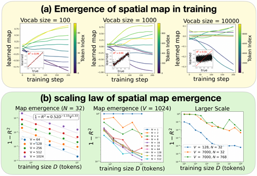
Figure 3. Spatial map emergence strongly depends on tokenization, and weakly on embedding dimensions. (a) Evolution of learned embeddings, i.e., token embeddings projected onto the best lin-early decodable direction at the last step (200). From left to right: vocabulary size \(V = 100,1000,10000\). Each inset shows the true coordinate and the learned coordinate. The spatial map emerges easily for a small vocabulary size \(V\) , but becomes poorly emergent for large \(V\) . (b) Spatial map quality, measured by \(R^2\) between the true coordinate and the learned coordinate. Left: \(1 − R^2\) obeys a scaling law with respect to vocabulary size V and training tokens D. Middle: \(R^2\) saturates when the embedding dimension \(N\) is beyond a critical value at 8. Right: Scaling up \(V\) or \(N\) does not improve, but actually harms spatial map emergence.
図3. 空間マップの出現はトークン化に大きく依存し、埋め込み次元には弱く依存する。(a) 学習済み埋め込みの進化、すなわち最終ステップ(200)における最適な線形デコード可能な方向に投影されたトークン埋め込み。左から右へ:語彙サイズ \(V = 100,1000,10000\)。各インセットは、真の座標と学習済み座標を示している。語彙サイズ \(V\) が小さい場合、空間マップは容易に出現するが、 \(V\) が大きい場合、空間マップの出現は困難になる。(b) 真の座標と学習済み座標の間の \(R^2\) で測定された空間マップの品質。左: \(1 − R^2\) は語彙サイズ V とトレーニング トークン D に関してスケーリング則に従います。中央: \(R^2\) は、埋め込み次元 \(N\) が 8 の臨界値を超えると飽和します。右: \(V\) または \(N\) を拡大しても空間マップの出現は改善されず、むしろ悪影響を及ぼします。
Smaller vocabulary size V improves emergence Fig-ure 3(a) shows the training dynamics of embedding pro-jections onto the best linear direction. For a fixed amount of data (\(D = 10^4\)), smaller vocabulary sizes produce signifi-cantly better spatial maps. Intuitively, larger vocabularies require proportionally more data to maintain adequate cov-erage before a spatial map can emerge.
語彙サイズVが小さいほど、出現率が向上する 図3(a)は、最適な線形方向への投影を埋め込む学習ダイナミクスを示しています。データ量が一定(\(D = 10^4\))の場合、語彙サイズが小さいほど、空間マップが大幅に改善されます。直感的に、語彙サイズが大きいほど、空間マップが出現するまでに適切なカバレッジを維持するために、比例して多くのデータが必要になります。
We fix \(N = 32\) and sweep \(V\) in \(\{64,128,256,512,1024\}\) and \(D_{traj}\) in \(\{64,128,256,512,1024\}\). The scaling law in Figure 3(b, left) fits well to
\[
1−R^2 \approx AD^{−αD} V^{αV}\quad (A = 0.52, α_D = 1.15, α_V = 1.33) \tag{1}
\]
with an excellent fit (\(R^2 \approx 0.995\)). Since \(α_V \geq α_D\), the training size \(D\) must increase at least as fast as the vocabu-lary size \(V\) to maintain comparable spatial-map quality.
非常に良好な適合度を示した(\(R^2 \approx 0.995\))。\(α_V \geq α_D\)であるため、同等の空間マップ品質を維持するためには、トレーニングサイズ\(D\)は語彙サイズ\(V\)と少なくとも同じ速さで増加する必要がある。
Embedding dimension \(N\) exhibits a critical value \(N_c\) One might expect that increasing the embedding dimen-sion \(N\) would help spatial map emergence, since higher-dimensional embeddings provide more “lottery tickets” for discovering a good linear direction. However, Figure 3(b, middle) shows that \(1 − R^2\) decreases with N only up to a critical value \(N_c \approx 8\), beyond which performance rapidly plateaus. Increasing \(N\) further offers little benefit.
埋め込み次元 \(N\) は臨界値 \(N_c\) を示す 高次元の埋め込みは良好な線形方向を発見するための「宝くじ券」をより多く提供するため、埋め込み次元 \(N\) を増やすと空間マップの出現に役立つと予想されるかもしれません。しかし、図3(b、中央) は、\(1 − R^2\) が臨界値 \(N_c \approx 8\) までしかNの増加とともに減少せず、それを超えると性能は急速に平坦化することを示しています。\(N\) をさらに増やしても、ほとんどメリットはありません。
Scaling up The above analyses use small-scale hyperparam-eters to allow sweeping many configurations efficiently. To connect more directly to the large-scale setup of Vafa et al. (2025), which uses \(V = 7000\) and \(N = 768\), we repeat our experiments with these values while sweeping \(D\) up to \(10^8\) tokens. Figure 3(b, right) shows that scaling slows markedly at large \(D\), suggesting diminishing returns once the data suf-ficiently cover the space. Moreover, comparing \(N = 768\) and \(N = 32\) (with \(V = 7000\) fixed) reveals that increasing N offers little improvement – and may even hinder – spatial map emergence. In contrast, reducing \(V\) to \(128\) produces a dramatic improvement.
スケールアップ 上記の分析では、小規模なハイパーパラメータを使用して、多くの構成を効率的にスイープできるようにしています。Vafa et al. (2025) の大規模セットアップ(\(V = 7000\) および \(N = 768\) を使用する)にさらに直接接続するために、\(D\) を \(10^8\) トークンまでスイープしながら、これらの値で実験を繰り返します。図 3(b、右) は、\(D\) が大きいとスケーリングが著しく遅くなることを示しており、データが十分に空間をカバーすると収穫逓減が起こることを示唆しています。さらに、\(N = 768\) と \(N = 32\)(\(V = 7000\) は固定)を比較すると、N を増やしても改善はほとんど見られず、空間マップの出現を妨げる可能性さえあることがわかります。対照的に、\(V\) を \(128\) に減らすと劇的な改善が得られます。
Take-home message Among all levers, reducing the vocab-ulary size \(V\) is the most effective way to improve spatial map emergence. However, choosing \(V\) too small leads to overly coarse binning, reducing the accuracy of predictions. An optimal intermediate choice of \(V\) should therefore bal-ance spatial-map quality and predictive resolution – an issue we investigate in the next section. Another natural solution would be using continuous coordinate without tokenization, but it would then face a spatial stability problem discussed in the next section.
まとめ あらゆる手段の中で、語彙サイズ \(V\) を小さくすることが、空間マップの出現率を向上させる最も効果的な方法です。しかし、 \(V\) を小さくしすぎると、ビニングが粗くなりすぎて予測精度が低下します。したがって、 \(V\) の最適な中間値は、空間マップの品質と予測解像度のバランスをとる必要があります。この問題については、次のセクションで検討します。もう1つの自然な解決策は、トークン化を行わずに連続座標を使用することですが、その場合は次のセクションで説明する空間安定性の問題に直面することになります。
Inductive Bias 1: Spatial smoothness 帰納バイアス1: 空間的滑らかさ
Failure mode: Vafa et al. (2025)’s transformer fails to learn a spatial map in the embedding space.
失敗モード: Vafa et al. (2025)のトランスフォーマーは埋め込み空間内の空間マップを学習できない。
Solution: (1) choose a smaller vocabulary size for tokenization, or (2) use continuous coordinates with-out tokenization. With (2), the spatial map is by default contained in the input.
解決策: (1) トークン化に使用する語彙サイズを小さくするか、(2) トークン化せずに連続座標を使用する。(2) の場合、空間マップはデフォルトで入力に含まれます。
Following the setup of Vafa et al. (2025), we have so far treated trajectory prediction as a classification problem by discretizing continuous spatial coordinates into discrete to-kens. A natural question is whether we can instead use continuous spatial coordinates directly as inputs, thereby eliminating the need to learn a spatial map altogether. Al-though Vafa et al. (2025) reported that discretized coordi-nates with cross-entropy loss (classification) outperform continuous coordinates with MSE loss (regression), we ar-gue that the continuous formulation merits further investiga-tion. To examine this question systematically, we introduce the Kepler dataset—a simplified benchmark consisting of idealized planetary orbits. On this controlled testbed, we directly compare two formulations: next-state prediction (regression) and next-token prediction (classification).
Vafa et al. (2025)の設定に従い、これまで連続空間座標を離散トークンに離散化することにより、軌道予測を分類問題として扱ってきました。当然の疑問として、連続空間座標を直接入力として使用し、空間マップを学習する必要性をまったくなくすことができるかどうかが挙げられます。Vafa et al. (2025)は、クロスエントロピー損失のある離散化座標 (分類) が MSE 損失のある連続座標 (回帰) よりも優れていると報告していますが、私たちは連続的な定式化をさらに調査する価値があると主張します。この問題を体系的に検討するために、理想化された惑星軌道で構成される簡略化されたベンチマークである Kepler データセットを導入します。この制御されたテストベッドで、次の状態予測 (回帰) と次のトークン予測 (分類) という 2 つの定式化を直接比較します。
Kepler dataset The Kepler dataset consists of 2D elliptical orbits of a planet around a central body (the sun) fixed at the origin. Each trajectory is generated by numerically integrating the gravitational equation of motion,
ケプラーデータセット ケプラーデータセットは、原点に固定された中心天体(太陽)の周りを回る惑星の2次元楕円軌道から構成されています。各軌道は、重力運動方程式を数値積分することによって生成されます。
\[
\frac{d^2\vec{r}}{dt^2}=-GM\frac{\vec{r}}{||\vec{r}||^3} \tag{2}
\]
where \(\vec{r} = (x,y)\) is the position vector and \(GM = 1.0\) is the gravitational parameter. For each trajectory, we initialize the system at perihelion (closest approach) with orbital param-eters sampled uniformly: eccentricity \(e ∈ [0.0,0.8]\), semi-major axis \(a ∈ [0.5,2.0]\), and initial orientation \(θ ∈ [0,2π]\). The initial position and velocity are computed from these parameters and then rotated by \(θ).
ここで、\(\vec{r} = (x,y)\) は位置ベクトル、\(GM = 1.0\) は重力パラメータです。各軌道において、近日点(最接近点)において、軌道パラメータ(離心率 \(e ∈ [0.0,0.8]\)、軌道長半径 \(a ∈ [0.5,2.0]\)、初期姿勢 \(θ ∈ [0,2π]\))を一様にサンプリングして系を初期化します。初期位置と速度はこれらのパラメータから計算され、\(θ) 回転されます。
We integrate the system using solve ivp in scipy with relative and absolute tolerances of \(10^{−8}\), sampling \(100\) equally spaced time points at a step size \(∆t = 0.2\). The resulting dataset contains \(D_{traj}\) trajectories (equivalently \(D = 100D_{traj}\) tokens), each providing a sequence of \((x,y)\) positions of shape \((100,2)\) that captures the full elliptical motion of the planet around the sun.
scipyのsolve ivpを用いて、相対および絶対許容誤差を\(10^{−8}\)としてシステムを積分し、ステップサイズ\(∆t = 0.2\)で等間隔の時点\(100\)をサンプリングします。結果として得られるデータセットには、\(D_{traj}\)個の軌跡(\(D = 100D_{traj}\)個のトークンと同等)が含まれ、各軌跡は、太陽の周りを周回する惑星の完全な楕円運動を捉える、形状\((100,2)\)の\((x,y)\)位置のシーケンスを提供します。
As discussed above, using continuous spatial coordinates as inputs naturally removes the need to learn a spatial map. However, this comes at a cost: the regression formulation is considerably more prone to error accumulation than its classification counterpart. It is well known that autoregres-sive models suffer from the spatial stability issue, i.e., error accumulates quickly at inference time; continuous variables exacerbate this issue because their outputs can become un-bounded. In contrast, discrete tokenization imposes a finite set of possible outputs, providing a form of “error correction” by projecting predictions back onto a discrete vocabulary. Perhaps for this reason, Vafa et al. (2025) reported that “we experimented between using (a) continuous coordinates (and MSE loss) and (b) discretized coordinates (with cross-entropy loss), finding the latter worked better.”
上で述べたように、連続空間座標を入力として使用すると、空間マップを学習する必要がなくなります。しかし、これには代償が伴います。回帰定式化は、分類モデルよりも誤差が蓄積されやすい傾向がかなり強いのです。自己回帰モデルは空間安定性の問題、つまり推論時に誤差が急速に蓄積されることはよく知られています。連続変数は出力が無限大になる可能性があるため、この問題を悪化させます。対照的に、離散トークン化は可能な出力の有限集合を課し、予測を離散語彙に投影することで、一種の「誤差補正」を提供します。おそらくこの理由から、Vafa et al. (2025) は、「(a) 連続座標(およびMSE損失)と (b) 離散化座標(クロスエントロピー損失あり)の使用を実験し、後者の方が効果的であることがわかった」と報告しています。
Below, we (1) identify the failure mode associated with regression and (2) introduce a mitigation strategy.
以下では、(1)回帰に関連する障害モードを特定し、(2)軽減戦略を紹介します。
A failure mode: error accumulation As shown in Figure 4 (leftmost, \(σ = 0.0\)), we condition on the first 50 points of a trajectory and autoregressively generate the next 50 points, comparing them with the true trajectory. Although the initial prediction error is small, it accumulates rapidly and causes catastrophic divergence, often sending the planet into the sun or off to infinity.
失敗モード:誤差の蓄積 図4(左端、σ = 0.0)に示すように、軌道の最初の50点を条件として、次の50点を自己回帰的に生成し、真の軌道と比較します。初期の予測誤差は小さいものの、急速に蓄積して壊滅的な発散を引き起こし、惑星を太陽に衝突させたり、無限遠に飛ばしたりすることがしばしばあります。
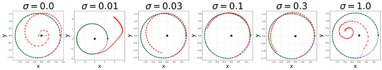
Figure 4. Error accumulation and fixing it by adding context noise in training. Each subplot shows the ground truth trajectory (blue solid circle), conditioning 50 points (green), and the generated 50 points (red). From left to right: training with different levels of context noise \(σ\). Naively training a regression-based transformer leads to severe error accumulation (left, \(σ = 0\)), whereas adding a reasonable amount of noise \(σ\) (e.g., \(σ = 0.1\)) to contexts during training substantially improves robustness.
図4. エラーの蓄積と、トレーニング中にコンテキストノイズを追加することでその修正を行う様子。各サブプロットは、グラウンドトゥルースの軌跡(青い実線)、コンディショニング後の50点(緑)、生成された50点(赤)を示しています。左から右へ:異なるレベルのコンテキストノイズ \(σ\) を使用したトレーニング。回帰ベースのトランスフォーマーを単純にトレーニングすると、深刻なエラー蓄積が発生します(左、\(σ = 0\))。一方、トレーニング中にコンテキストに適度な量のノイズ \(σ\)(例:\(σ = 0.1\))を追加すると、堅牢性が大幅に向上します。
Fix: noisy context learning To make the generation process more robust, the model must be trained to handle deviations from perfect past contexts. To simulate such deviations, we add Gaussian noise to the historical inputs during training, leading to the modified objective
修正:ノイズの多いコンテキスト学習 生成プロセスをより堅牢にするためには、モデルが過去の完全なコンテキストからの逸脱を処理できるように訓練される必要がある。このような逸脱をシミュレートするために、訓練中に過去の入力にガウスノイズを追加することで、修正された目的関数が得られる。
\[
L = \sum_{i=1}^N ||\vec{r}_{i+1}− f_θ(\vec{r}_i + σ\vec{ϵ}_i, ···, \vec{r}_0 + σ\vec{ϵ}_0)||^2 \tag{3}
\]
where \(\vec{ϵ}_i \sim \mathcal{N}(0,\mathbf{I}_2)\) is drawn from a normal distribution. This is a technique known as noisy context learning (Ren et al., 2025). Figure 4 shows that an intermediate noise level (σ = 0.1) yields the most accurate predictions: too little noise fails to counteract error accumulation, while too much noise overwhelms the learning signal.
ここで、\(\vec{ϵ}_i \sim \mathcal{N}(0,\mathbf{I}_2)\)は正規分布から抽出されます。これはノイズコンテキスト学習(Ren et al., 2025)として知られる手法です。図4は、中程度のノイズレベル(σ = 0.1)で最も正確な予測が得られることを示しています。ノイズが少なすぎると誤差の蓄積を抑えることができず、ノイズが多すぎると学習信号を圧倒してしまいます。
To fairly compare regression and classification models, two subtleties must be addressed. (1) Hyperparameter choices.
回帰モデルと分類モデルを公平に比較するためには、2つの微妙な点に対処する必要があります。(1) ハイパーパラメータの選択。
We have shown that vocabulary size \(V\) is a crucial hyperpa-rameter for classification, while the noise scale σ strongly affects regression performance. Thus, for each method, we sweep over the relevant hyperparameters and report the per-formance of the best model. (2) Evaluation metric. Because classification models are trained with cross-entropy loss and regression models with MSE loss, their training losses are not directly comparable. Instead, we convert predicted to-kens into continuous coordinates \((x,y)\) by mapping each token to the center of its corresponding bin. Using the first 50 points as context, we autoregressively generate the next 50 points. The evaluation metric is the mean distance er-ror, defined as the Euclidean distance between generated and ground-truth positions, averaged over the 50 gener-ated points. Detailed training dynamics are included in Appendix B.2 (classification) and B.3 (regression).
語彙サイズ \(V\) は分類にとって重要なハイパーパラメータであり、ノイズスケール σ は回帰のパフォーマンスに強く影響することを示しました。したがって、各方法について、関連するハイパーパラメータをスイープし、最良のモデルのパフォーマンスを報告します。 (2) 評価指標。分類モデルはクロスエントロピー損失でトレーニングされ、回帰モデルは MSE 損失でトレーニングされるため、トレーニング損失を直接比較することはできません。代わりに、各トークンを対応するビンの中心にマッピングすることにより、予測トークンを連続座標 \((x,y)\) に変換します。最初の 50 ポイントをコンテキストとして使用して、次の 50 ポイントを自己回帰的に生成します。評価指標は平均距離誤差であり、生成された位置と真の位置間のユークリッド距離として定義され、生成された 50 ポイントで平均されます。詳細なトレーニングダイナミクスは、付録 B.2 (分類) および B.3 (回帰) に含まれています。
Figure 5 reports the mean distance error for both regression and classification models. In the left panel, we confirm that an intermediate noise scale \(σ\) yields the best regression performance. In the middle panel, we observe a sweet spot for vocabulary size \(V\) , with the optimal \(V\) increasing with the training size \(D\) In the right panel, regression models (solid green) consistently outperform classification models (solid blue) across all training sizes when hyperparameters are optimized (choosing \(V\) for classification and \)σ\) for re-gression). However, if \(σ\) is naively fixed to zero, regression models (dashed green) may underperform the best classifi-cation models (solid blue) at large training sizes – precisely the regime considered by Vafa et al. (2025).
図 5 は、回帰モデルと分類モデルの両方の平均距離誤差を示しています。左のパネルでは、中間のノイズ スケール \(σ\) が最良の回帰パフォーマンスをもたらすことが確認できます。中央のパネルでは、語彙サイズ \(V\) のスイート スポットが見られ、最適な \(V\) はトレーニング サイズ \(D\) とともに増加します。右のパネルでは、ハイパーパラメータが最適化されている場合 (分類には \(V\) を選択し、回帰には \)σ\) を選択)、回帰モデル (実線の緑) はすべてのトレーニング サイズで分類モデル (実線の青) を一貫して上回っています。ただし、\(σ\) が単純に 0 に固定されると、回帰モデル (破線の緑) は大規模なトレーニング サイズで最良の分類モデル (実線の青) を下回る可能性があります。これはまさに Vafa ら (2025) が検討した状況です。
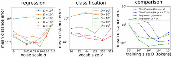
Figure 5. Comparing regression and classification transformers (\(D\): training tokens), using mean distance error as the metric to evaluate predictive performance. Left: regression models exhibit a sweet spot in the context noise scale \(σ\). Middle: regression models also exhibit a sweet spot in the vocabulary size \(V\). Right: comparing regression and classification across different training data sizes \(D\). Regression models consistently outperform classification models when their best hyperparameters (\(σ\) or \(V\) ) are selected. However, naively trained regression models (\(σ = 0\)) underperform the best classification models when the training data is large.
図5. 回帰トランスフォーマーと分類トランスフォーマー(\(D\): トレーニングトークン)の比較。平均距離誤差を予測性能評価指標として使用しています。左:回帰モデルはコンテキストノイズスケール\(σ\)においてスイートスポットを示しています。中央:回帰モデルは語彙サイズ\(V\)においてもスイートスポットを示しています。右:異なるトレーニングデータサイズ\(D\)における回帰と分類の比較。回帰モデルは、最適なハイパーパラメータ(\(σ\)または\(V\))が選択された場合、一貫して分類モデルよりも優れたパフォーマンスを発揮します。しかし、単純にトレーニングされた回帰モデル(\(σ = 0\))は、トレーニングデータが大きい場合、最適な分類モデルよりもパフォーマンスが低くなります。
Inductive Bias 2: Spatial Stability 帰納バイアス2: 空間的安定性
Failure mode: Transformers (auto-regressive mod-els in general) accumulate errors fast, especially for unbounded continuous variables.
失敗モード: トランスフォーマー(一般的には自己回帰モデル)は、特に無制限の連続変数の場合、エラーが急速に蓄積されます。
Solution: forcing the model to correct errors in in-ference by adding input perturbations in training. As a result, regression models with continuous inputs outperform classification models with tokenization.
解決策: 学習時に入力摂動を加えることで、モデルに推論エラーの修正を強制する。その結果、連続入力を用いた回帰モデルは、トークン化を用いた分類モデルよりも優れた性能を示す。
Having established in the previous sections that regression models have two key advantages over classification mod-els – (1) they naturally preserve spatial continuity without needing to learn a spatial map, and (2) they can achieve lower mean prediction error—we now return to the central question: do regression transformers learn a Newtonian world model? There is one more inductive bias needed – temporal locality. We note that Newtonian mechanics is a second-order differential equation, meaning that the next state depends only on the current state and the previous state, but not on other states before that. This suggests using a context length of 2. This motivates us to vary context length to control temporal locality.
前のセクションで、回帰モデルには分類モデルに比べて 2 つの重要な利点がある (1) 空間マップを学習する必要がなく、空間の連続性を自然に維持できること、(2) 平均予測誤差を低く抑えられること、を確認しました。ここで中心的な疑問、「回帰トランスフォーマーはニュートン世界モデルを学習するのか?」に戻ります。もう 1 つの帰納バイアス、つまり時間的局所性が必要です。ニュートン力学は 2 階微分方程式であり、次の状態は現在の状態と前の状態にのみ依存し、それ以前の状態には依存しないことに注意してください。これはコンテキスト長を 2 にすることを示唆しています。これが、時間的局所性を制御するためにコンテキスト長を変化させる動機となります。
Newtonian world model We apply linear probing to search for linear directions in the model’s latent representations that correlate with force variables: force magnitude \(F ≡ ||\vec{F}||\), the \(x\)-component \(F_x\), and the \(y\)-component \(F_y\). We probe a wide range of internal activations, including the inputs and outputs of attention and MLP blocks (both before and after residual merging), as well as hidden states inside MLP modules. For each force-related target, we report the highest R2 across all layers (Results for R2 of each layer are included in Appendix C). Figure 6(a) (green bars) reveals that while context length 100 partially captures these force variables (\(R^2 \approx 0.9\)), only context length 2 yields a precise representation \(R^2 \approx 0.999\).
ニュートン世界モデル 線形プローブを用いて、力の変数(力の大きさ \(F ≡ ||\vec{F}||\)、\(x\)成分 \(F_x\)、\(y\)成分 \(F_y\))と相関するモデルの潜在表現における線形方向を探索する。アテンションブロックとMLPブロックの入力と出力(残差マージの前後の両方)、MLPモジュール内の隠れ状態など、広範囲の内部活性化をプローブする。各力関連のターゲットについて、全層で最高のR2を報告している(各層のR2の結果は付録Cに含まれます)。図6(a)(緑のバー)は、コンテキスト長100でこれらの力の変数を部分的に捉えている(\(R^2 \approx 0.9\))一方、コンテキスト長2でのみ正確な表現\(R^2 \approx 0.999\)が得られることを示しています。
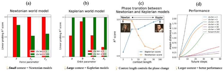
Figure 6. The tale of two world models – the context length controls the transformer to learn a Newtonian model or a Keplerian model. (a) Small context lengths (e.g., 2) lead to Newtonian models, with transformers internally computing gravitational forces. (b) Long context lengths (e.g., 100) lead to Keplerian models, with transformers internally computing orbit parameters (semi-major/minor-axis length a/b, Laplace-Runge-Lenz vector A). (c) Varying context lengths controls the phase transition between Newtonian vs Keplerian world models. (d) Mean distance error as a function of future steps and context lengths. Larger context lengths lead to improved predictive performance (lower errors).
図6. 2つの世界モデルの物語 – コンテキスト長は、トランスフォーマーがニュートンモデルまたはケプラーモデルのどちらを学習するかを制御します。(a) コンテキスト長が短い(例:2)場合はニュートンモデルとなり、トランスフォーマーは内部で重力を計算します。(b) コンテキスト長が長い(例:100)場合はケプラーモデルとなり、トランスフォーマーは内部で軌道パラメータ(軌道長半径/短半径a/b、ラプラス・ルンゲ・レンツベクトルA)を計算します。(c) コンテキスト長の変化は、ニュートン世界モデルとケプラー世界モデル間の位相遷移を制御します。(d) 平均距離誤差は、将来のステップとコンテキスト長の関数として表されます。コンテキスト長が大きいほど、予測性能が向上します(誤差が低くなります)。
Keplerian world model This raises the question: what world model does a transformer learn when the context length is large? It is obvious that the model must have learned something meaningful in order to make accurate predictions. If we adopt Kepler’s geometric perspective orbits are ellipses (Kepler’s first law), we can first fit an elliptical equation based on all previous points and then predict the next state by continuing the curve. We refer to this global geometric approach as Keplerian world model, in contrast to Newtonian world model based on force com-putations (see Figure 1 right for illustrations). To test this hypothesis, we probe the model for key geometric param-eters of ellipses: semi-major axis a, semi-minor axis b, Laplace–Runge–Lenz vector \(\vec{A} = (A_x,A_y)\). Figure 6(b) shows that these geometric quantities are linearly encoded almost perfectly (\(R^2 \approx 0.998\)) when the context length is 100, whereas they are relatively poor (\(R^2 \approx 0.9\)) when the context length is 2. There is a phase transition between Ke-plerian and Newtonian models by varying context lengths, as shown in Figure 6(c) – while transformers with small context lengths preferentially learn Newtonian world mod-els, transformers with large context lengths preferentially learn Keplerian world models. Furthermore, Figure 6(d) shows that larger context lengths achieve lower prediction error, because the Keplerian model (global, geometry-based) is more robust to noise than the Newtonian model (local, force-based), hence making more accurate long-horizon predictions.
ケプラーの世界モデル これにより、コンテキスト長が大きい場合、トランスフォーマーはどのような世界モデルを学習するのかという疑問が生じます。正確な予測を行うためには、モデルが何か意味のあることを学習している必要があることは明らかです。ケプラーの幾何学的視点、軌道は楕円形 (ケプラーの第一法則) を採用すると、まず以前のすべての点に基づいて楕円方程式を近似し、次に曲線を継続することで次の状態を予測できます。このグローバルな幾何学的アプローチを、力の計算に基づくニュートンの世界モデルとは対照的に、ケプラーの世界モデルと呼びます (図1右を参照)。この仮説を検証するために、楕円の主要な幾何学的パラメータ、長半径 a、短半径 b、ラプラス・ルンゲ・レンツ ベクトル \(\vec{A} = (A_x,A_y)\) についてモデルをプローブします。図6(b)は、コンテキスト長が100の場合、これらの幾何学的量がほぼ完璧に線形エンコードされている(\(R^2 \approx 0.998\))のに対し、コンテキスト長が2の場合は比較的劣っている(\(R^2 \approx 0.9\))ことを示しています。図6(c)に示すように、コンテキスト長を変えることで、ケプラーモデルとニュートンモデルの間に位相遷移があります。コンテキスト長が小さいトランスフォーマーはニュートン世界モデルを優先的に学習しますが、コンテキスト長が大きいトランスフォーマーはケプラー世界モデルを優先的に学習します。さらに、図6(d)は、コンテキスト長が大きいほど予測誤差が低くなることを示しています。これは、ケプラーモデル(グローバル、幾何学ベース)はニュートンモデル(ローカル、力ベース)よりもノイズに対して堅牢であるため、より正確な長期予測を行うためです。
Inductive Bias 3: Temporal Locality 帰納バイアス3: 時間的局所性
Failure mode: A regression transformer fails to learn the Newtonian model when the context length is too large.
失敗モード:コンテキスト長が長すぎる場合、回帰トランスフォーマーはニュートンモデルを学習できません。
Solution: Reducing the context length to 2 induces a Newtonian model. Short context lengths induce the Newtonian model, while long context lengths induce the Keplerian model.
解決策:コンテキスト長を2に減らすと、ニュートンモデルが誘導されます。コンテキスト長が短い場合はニュートンモデルが誘導され、コンテキスト長が長い場合はケプラーモデルが誘導されます。
The goal of this paper is to identify failure modes that pre-vent current foundation models from learning “world mod-els,” using a controlled setup based on synthetic planetary motion data. We find that Vafa et al. (2025) fails to learn a spatial map due to its tokenization scheme. After addressing this issue—either by reducing the vocabulary size or by using regression models trained with MSE loss—Newton’s world model still does not emerge. Instead, a geometric approach that fits ellipses (Kepler’s world model) emerges. Newton’s world model appears only when the block size is reduced to 2, consistent with the fact that Newtonian mechanics is a second-order dynamical system. Our find-ings underscore the challenges and subtleties involved in inducing even very simple world models (such as planetary motion) in transformer architectures.
本論文の目的は、合成惑星運動データに基づく制御されたセットアップを使用して、現在の基礎モデルが「世界モデル」を学習するのを妨げる失敗モードを特定することです。Vafa et al. (2025) は、トークン化スキームのために空間マップを学習できないことがわかりました。語彙サイズを削減するか、MSE損失でトレーニングされた回帰モデルを使用することによってこの問題に対処した後でも、ニュートンの世界モデルはまだ出現しません。代わりに、楕円に適合する幾何学的アプローチ (ケプラーの世界モデル) が出現します。ニュートンの世界モデルは、ブロックサイズが2に縮小された場合にのみ出現し、ニュートン力学が2次の動的システムであるという事実と一致しています。私たちの発見は、トランスフォーマーアーキテクチャで非常に単純な世界モデル (惑星運動など) を誘導することに伴う課題と微妙な点を強調しています。
Finally, our results offer a critical perspective on the defini-tion of “world models” in artificial intelligence. Please refer to Appendix A for a summary of previous definitions. While prevailing views often characterize a world model purely by its predictive utility—the ability to simulate future states given an action—we argue that prediction is necessary but not sufficient. As our “Keplerian” models demonstrate, a system can achieve high predictive accuracy by merely fitting complex curves to historical data, effectively mem-orizing the training distribution. However, true scientific understanding requires discovering the governing mechanisms — the simple, invariant laws (like \(F = ma\)) that generate the data.
最後に、我々の研究結果は、人工知能における「世界モデル」の定義に批判的な視点を提示する。これまでの定義の概要については付録Aを参照のこと。一般的な見解では、世界モデルは予測の有用性、つまり行動を与えられた場合に将来の状態をシミュレートする能力のみによって特徴付けられることが多いが、我々は予測は必要だが十分ではないと主張している。我々の「ケプラー」モデルが示すように、システムは過去のデータに複雑な曲線を当てはめ、トレーニング分布を効果的に記憶するだけで、高い予測精度を達成できる。しかし、真の科学的理解には、データを生成する支配的なメカニズム、つまり単純で不変の法則(\(F = ma\)など)を発見する必要がある。
We speculate that this mechanistic understanding is the prerequisite for radical out-of-distribution (OOD) gen-eralization. A curve-fitter (Kepler) is bound to the “grey elephants” (familiar trajectories) it has seen; it cannot reli-ably predict the behavior of a “pink elephant”—a scenario strictly outside its training data. In contrast, a mechanistic model (Newton) decouples the rule from the history. Be-cause it understands the causal invariant (\(F = ma\)), it can correctly predict the future of a pink elephant just as accu-rately as a grey one. Our work suggests that for AI to evolve from a predictor to a scientist, we must architecturally con-strain it to look for these simple, local mechanisms rather than complex global histories.
このメカニズムの理解は、ラジカル分布外(OOD)一般化の前提条件であると推測しています。カーブフィッター(ケプラー)は、これまで見てきた「灰色の象」(馴染みのある軌跡)に縛られており、「ピンクの象」の行動、つまりトレーニングデータの範囲外のシナリオを確実に予測することはできません。対照的に、メカニズムモデル(ニュートン)は、ルールを履歴から切り離します。因果不変量(\(F = ma\))を理解しているため、ピンクの象の未来を灰色の象と同じくらい正確に予測できます。私たちの研究は、AIが予測者から科学者へと進化するためには、複雑なグローバル履歴ではなく、これらの単純でローカルなメカニズムを探すようにアーキテクチャ的に制約する必要があることを示唆しています。
Limitations (1) For simplicity, we have simplified the setup of Vafa et al. (Vafa et al., 2025) by using one time-scale (they used two time-scales). (2) We used linear probes to verify the existence of world models, but this method yields only implicit knowledge: the network “knows” Force, but does not explicitly output Newton’s equations. Furthermore, probing requires us to know what to look for a priori. A fully autonomous “AI Physicist” would require an additional mechanism—such as a secondary “interpreter” network or symbolic regression head—that actively searches the latent space for simple, linear relationships to automatically ex-tract and output symbolic laws like \(F = ma\) without human supervision. Related works about “AI Physicists” are re-viewed in Appendix A – although they have proven useful in highly-controlled setups where carefully designed specialist models are employed, end-to-end extraction of clean and simple laws (if they do exist) from black-box foundation laws remains a challenging but urgent direction.
制限 (1) 簡潔にするために、Vafa et al. (Vafa et al., 2025) のセットアップを 1 つのタイムスケール (彼らは 2 つのタイムスケールを使用) に簡略化しました。 (2) 世界モデルの存在を確認するために線形プローブを使用しましたが、この方法は暗黙の知識しか生成しません。つまり、ネットワークは Force を「知っている」ものの、ニュートン方程式を明示的に出力しません。さらに、プローブ処理では、何を事前に探すべきかを知っている必要があります。完全に自律的な「AI 物理学者」には、二次的な「インタープリター」ネットワークやシンボリック回帰ヘッドなどの追加のメカニズムが必要になります。このメカニズムは、人間の監視なしに \(F = ma\) のようなシンボリック法則を自動的に抽出して出力するために、潜在空間で単純な線形関係を積極的に検索します。 「AI物理学者」に関する関連研究は付録Aで再検討されています。これらは、慎重に設計された専門モデルが採用されている高度に制御された設定では有用であることが証明されていますが、ブラックボックスの基礎法則からクリーンでシンプルな法則(存在する場合)をエンドツーエンドで抽出することは、依然として困難ですが緊急の課題です。
We would like to thank Liam Storan for the helpful discus-sion. S.G thanks the Simons Collaboration on the Physics of Learning and Neural Computation and a Schmidt Sciences Polymath award for funding. Z.L, S.S and A.T thank The James Fickel Enigma Project Fund.
有益な議論をしてくださったLiam Storan氏に感謝します。S.Gは、学習物理学と神経計算に関するSimons Collaborationと、資金提供をいただいたSchmidt Sciences Polymath賞に感謝します。Z.L、S.S、A.Tは、James Fickel Enigma Project Fundに感謝します。
World models The notion of “world models” has appeared across several threads in machine learning, generally referring to internal representations/computations that capture the dynamics or structure of an environment. Early work in model-based reinforcement learning developed predictive latent-state models for planning and control, such as the World Models framework of Ha and Schmidhuber (Ha & Schmidhuber, 2018), PlaNet (Hafner et al., 2019b), and Dreamer (Hafner et al., 2019a), which learn compact dynamic models from pixel observations. A parallel line of work in neuroscience-inspired ML explores generative predictive coding frameworks and latent dynamics models as computational analogues of internal world representations (Rao & Ballard, 1999; Friston, 2010; Lotter et al., 2017). More recently, the emergence of world models in large foundation models has attracted growing attention: language models have been shown to encode linearizable geometric or semantic structures (Gurnee & Tegmark, 2024; Park et al., 2024; Korchinski et al., 2025), vision-language models capture rich conceptual relationships (Radford et al., 2021; Goh, 2021; Alayrac et al., 2022), and multimodal agents acquire implicit affordances for acting in embodied environments (Zitkovich et al., 2023; Reed et al., 2022; Kim et al., 2024).
世界モデル 「世界モデル」という概念は、機械学習のさまざまな分野で登場しており、一般的には環境のダイナミクスや構造を捉える内部表現/計算を指します。モデルベース強化学習の初期の研究では、計画と制御のための予測潜在状態モデルが開発されました。例えば、HaとSchmidhuberの世界モデルフレームワーク(Ha & Schmidhuber, 2018)、PlaNet(Hafner et al., 2019b)、Dreamer(Hafner et al., 2019a)は、ピクセル観測からコンパクトな動的モデルを学習します。神経科学に着想を得た機械学習における並行した研究では、生成予測符号化フレームワークと潜在ダイナミクスモデルを、内部世界表現の計算類似物として研究しています(Rao & Ballard, 1999; Friston, 2010; Lotter et al., 2017)。最近では、大規模な基礎モデルにおける世界モデルの出現がますます注目を集めています。言語モデルは線形化可能な幾何学的構造や意味的構造をエンコードすることが示されており (Gurnee & Tegmark, 2024; Park et al., 2024; Korchinski et al., 2025)、視覚言語モデルは豊富な概念的関係を捉え (Radford et al., 2021; Goh, 2021; Alayrac et al., 2022)、マルチモーダルエージェントは具現化された環境で動作するための暗黙的なアフォーダンスを獲得します (Zitkovich et al., 2023; Reed et al., 2022; Kim et al., 2024)。
AI physicists Within physics and scientific modeling, AI physicist approaches have demonstrated that symbolic laws and interpretable dynamical equations can emerge from neural network training (Wu & Tegmark, 2019; Brunton et al., 2016; Cranmer et al., 2020; Lemos et al., 2023; Liu & Tegmark, 2021; Liu et al., 2022; 2024; Udrescu & Tegmark, 2020), suggesting that data-driven models can recover ground-truth world structures under the right inductive biases. Crucially, these methods typically impose strong structural priors (e.g., sparsity, symmetry, or graph structure). This leaves open the question of whether general-purpose architectures like Transformers can recover such ”world models” without these domain-specific constraints. Recent work by Vafa et al. (Vafa et al., 2025) suggests they cannot, reporting negative results even on simple planetary-motion datasets. Our work builds on these lines of inquiry but demonstrates that recovering true physical laws does not require strong symbolic priors, but rather a minimal assumption of locality—the intuitive idea that nature is governed by simple local rules rather than a complex history of the past. By constraining the model to seek such simple explanations, we show that general-purpose architectures can recover the ground-truth world structure without domain-specific constraints.
AI 物理学者 物理学と科学的モデリングにおいて、AI 物理学者のアプローチは、ニューラル ネットワークのトレーニングから記号法則と解釈可能な動的方程式が出現できることを実証しました (Wu & Tegmark, 2019; Brunton et al., 2016; Cranmer et al., 2020; Lemos et al., 2023; Liu & Tegmark, 2021; Liu et al., 2022; 2024; Udrescu & Tegmark, 2020)。これは、データ駆動型モデルが適切な帰納バイアスの下で真の世界構造を回復できることを示唆しています。重要なのは、これらの手法が通常、強力な構造的事前条件 (スパース性、対称性、グラフ構造など) を課すことです。これにより、Transformer などの汎用アーキテクチャがこれらのドメイン固有の制約なしにそのような「世界モデル」を回復できるかどうかという疑問が残ります。Vafa らによる最近の研究(Vafa et al., 2025)は、単純な惑星運動データセットでさえ否定的な結果を報告しており、それらは不可能であることを示唆しています。私たちの研究はこれらの研究を基にしていますが、真の物理法則を復元するには、強力な記号的事前分布ではなく、最小限の局所性仮定、つまり自然は過去の複雑な歴史ではなく、単純な局所的ルールによって支配されているという直感的な考え方が必要であることを示しています。モデルをそのような単純な説明を求めるように制約することで、汎用アーキテクチャがドメイン固有の制約なしに真の世界構造を復元できることを示します。
In the main paper, for the 1D sine-wave dataset, we report the best (lowest) value of \(1 − R^2\) attained during training. This choice is necessary because the optimal mapping is not always achieved at the final training step: the training dynamics can exhibit non-monotonic behavior due to overfitting. Figure 7 illustrates the evolution of the training loss, test loss, and map quality \(R^2\) for different vocabulary sizes and numbers of training tokens. For small training budgets (e.g., \(10^4\) tokens), severe overfitting is observed, as evidenced by a large gap between the training and test losses. In this regime, both the test loss and the map quality evolve non-monotonically: they initially improve but subsequently degrade once overfitting sets in. Notably, with limited data, a smaller vocabulary size (\(V = 128\)) yields better maps than a larger one (\(V = 7000\)), highlighting the advantage of smaller vocabularies in the low-data regime. Larger vocabulary sizes require more data to avoid overfitting. For example, with \(10^6\) training tokens (middle column), the train–test gap is negligible for \(V = 128\) but remains noticeable for \(V = 7000\). However, larger vocabularies benefit from longer scaling as the training data increases: for \(V = 7000\), performance continues to improve when scaling from \(10^6\) to \(10^8\) tokens, whereas such gains largely saturate for \(V = 128\).
本論文では、1次元正弦波データセットにおいて、トレーニング中に達成された\(1 − R^2\)の最良(最低)値を報告しています。この選択は、最適なマッピングが必ずしも最終トレーニングステップで達成されるとは限らないため、必要となります。トレーニングダイナミクスは、過学習により非単調な挙動を示す可能性があります。図7は、異なる語彙サイズとトレーニングトークン数における、トレーニング損失、テスト損失、およびマップ品質\(R^2\)の変化を示しています。トレーニングバジェットが小さい場合(例えば、\(10^4\)トークン)、トレーニング損失とテスト損失の間に大きなギャップがあることから明らかなように、深刻な過学習が観察されます。この状況では、テスト損失とマップ品質はどちらも非単調に変化します。つまり、最初は改善しますが、その後、過学習が始まると低下します。特に、データが限られている場合、語彙サイズが小さい(\(V = 128\))方が、大きい(\(V = 7000\))よりもマップ品質が向上し、データ量が少ない状況では語彙数が少ないことの利点が強調されます。語彙数が多いほど、過学習を避けるために必要なデータ量が多くなります。例えば、トレーニングトークンが\(10^6\)の場合(中央の列)、トレーニングとテストのギャップは\(V = 128\)では無視できるほど小さいですが、\(V = 7000\)では依然として顕著です。ただし、トレーニング データが増えるにつれて、語彙が大きいほど、スケーリングが長くなるというメリットがあります。\(V = 7000\) の場合、\(10^6\) トークンから \(10^8\) トークンにスケーリングするとパフォーマンスが向上し続けますが、\(V = 128\) の場合、このようなゲインはほぼ飽和します。
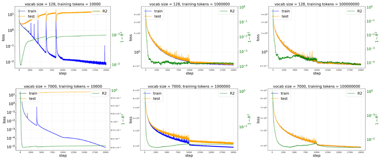
Figure 7. Training dynamics of the training loss, test loss, and \(R^2\) for the 1D sine-wave dataset, with vocabulary sizes 128,7000 and training token counts \(10^4,10^6,10^8\). When the training set is small, the learned map initially improves (lower \(1 − R^2\)) but subsequently degrades as overfitting sets in. Larger vocabulary sizes require more data to mitigate overfitting, as reflected by a larger train–test loss gap.
図7. 1次元正弦波データセットにおける、訓練損失、テスト損失、および\(R^2\)の訓練ダイナミクス。語彙サイズは128,7000、訓練トークン数は\(10^4,10^6,10^8\)。訓練セットが小さい場合、学習済みマップは当初は改善(\(1 − R^2\)が低い)しますが、その後、過学習が始まるにつれて劣化します。語彙サイズが大きいほど、過学習を軽減するためにより多くのデータが必要になり、訓練とテストの損失ギャップが大きくなります。
When we formulate the Kepler problem as a classification task (next-token prediction) trained with cross-entropy loss, two key hyperparameters are the vocabulary size and the number of training tokens. As shown in Figure 8, overfitting can occur when the training data are limited, especially for large vocabulary sizes. Although the model is trained using cross-entropy loss, we additionally compute an effective MSE loss defined by the squared distance between the center of the predicted token and the true next position. This allows for a fair comparison with the regression results shown in Figure 9.
ケプラー問題を、クロスエントロピー損失を用いて学習された分類タスク(次のトークン予測)として定式化すると、語彙サイズと学習トークン数という2つの重要なハイパーパラメータが重要になります。図8に示すように、学習データが限られている場合、特に語彙サイズが大きい場合、過学習が発生する可能性があります。モデルはクロスエントロピー損失を用いて学習されていますが、予測トークンの中心と真の次の位置との間の距離の2乗で定義される実効MSE損失も追加で計算します。これにより、図9に示す回帰結果と公平に比較することができます。
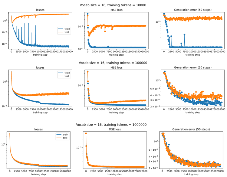
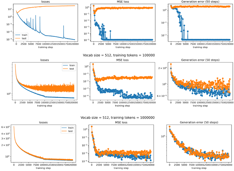
Figure 8. When formulating the Kepler problem as a classification task (next-token prediction), performance depends on both the vocabulary size and the number of training tokens. For each configuration, we plot the training dynamics of the cross-entropy loss, the effective MSE loss (defined as the squared distance between the true point and the center of the predicted token), and the generation distance error averaged over the next 50 steps. When the training data are limited, smaller vocabulary sizes yield better performance.
図8. ケプラー問題を分類タスク(次トークン予測)として定式化すると、パフォーマンスは語彙サイズとトレーニングトークン数の両方に依存します。各設定について、クロスエントロピー損失、実効MSE損失(真の点と予測トークンの中心間の距離の2乗として定義)、および次の50ステップで平均化された生成距離誤差のトレーニングダイナミクスをプロットします。トレーニングデータが限られている場合、語彙サイズが小さいほどパフォーマンスが向上します。
When we formulate the Kepler problem as a regression task (next-state prediction) trained using MSE loss, two key hyperparameters are the in-context noise level and the number of training tokens. As shown in Figure 9, overfitting can occur when the training data are limited; however, the amount of data required to avoid overfitting is smaller than in the classification setting shown in Figure 8. For example, with \(10^5\) training tokens, a noticeable train–test gap remains for classification, whereas it is negligible for regression. In addition, introducing a moderate level of in-context noise during training (\(σ\)) helps reduce generation error, as demonstrated in Figure 4.
Kepler問題をMSE損失を用いて学習する回帰タスク(次状態予測)として定式化すると、2つの重要なハイパーパラメータ、すなわちコンテキスト内ノイズレベルとトレーニングトークン数が重要になります。図9に示すように、トレーニングデータが限られている場合、オーバーフィッティングが発生する可能性があります。しかし、オーバーフィッティングを回避するために必要なデータ量は、図8に示した分類設定よりも少なくなります。例えば、トレーニングトークン数が\(10^5\)の場合、分類では顕著なトレーニングとテストのギャップが残りますが、回帰では無視できるほどです。さらに、トレーニング中に適度なレベルのコンテキスト内ノイズ(\(σ\))を導入すると、図4に示すように、生成エラーの低減に役立ちます。
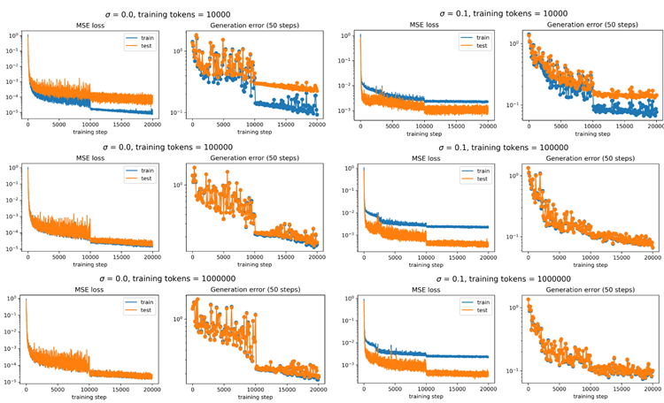
Figure 9. When formulating the Kepler problem as a regression task (next-state prediction), performance depends on both the noise scale and the number of training tokens. For each configuration, we plot the training dynamics of the MSE loss and the generation distance error averaged over the next 50 steps. Introducing a moderate level of in-context noise during training offers advantages over training without noise.
図9. ケプラー問題を回帰タスク(次状態予測)として定式化する場合、パフォーマンスはノイズスケールとトレーニングトークン数の両方に依存します。各設定について、次の50ステップにおける平均MSE損失と生成距離誤差のトレーニングダイナミクスをプロットします。トレーニング中に適度なレベルのコンテキスト内ノイズを導入すると、ノイズなしのトレーニングよりも優れた結果が得られます。
In the main paper, for the Kepler model, we showed that a transformer with a short context length (2) learns a Newtonian model, whereas a transformer with a long context length (100) learns a Keplerian model. What happens when we interpolate between these two extremes? Figure 10 shows that the transition is monotonic: increasing the context length yields models that are progressively more Keplerian and less Newtonian. For simplicity, the metrics in the rightmost plot are averaged across components (i.e., the Keplerian score averages over \(a,b,A_x,A_y\), while the Newtonian score averages over F,Fx,Fy).
本論文では、ケプラーモデルを用いて、コンテキスト長が短い(2)トランスフォーマーはニュートンモデルを学習し、コンテキスト長が長い(100)トランスフォーマーはケプラーモデルを学習することを示しました。これらの両極端の間を補間するとどうなるでしょうか?図10は、遷移が単調であることを示しています。コンテキスト長が長くなるにつれて、モデルは徐々にケプラー的になり、ニュートン的ではなくなります。簡略化のため、右端のグラフの指標はコンポーネント全体で平均化されています(つまり、ケプラースコアは\(a,b,A_x,A_y\) で平均化され、ニュートンスコアはF,Fx,Fy で平均化されます)。
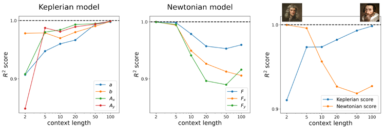
Figure 10. Effect of context length on the learned world model. Left: Larger context lengths favor the emergence of a Newtonian world model. Middle: Smaller context lengths favor the emergence of a Keplerian world model. Right: A summary plot obtained by averaging the \(R^2\) scores across different probing targets.
図10. 学習された世界モデルに対するコンテキスト長の影響。左:コンテキスト長が長いほど、ニュートン力学的な世界モデルの出現が促進される。中央:コンテキスト長が短いほど、ケプラー力学的な世界モデルの出現が促進される。右:異なるプロービングターゲット間の \(R^2\) スコアを平均して得られた要約プロット。
In the main paper, we report the best \(R^2\) over all hidden representations. But where are the best representations, and how do they emerge in forward computations? For context length 2, probing results are shown in Figure 11. For context length 100, probing results are shown in Figure 12. Besides the probing targets reported in the main paper, we compute other related quantities as well.
本論文では、すべての隠れ表現における最良の\(R^2\)を報告しました。しかし、最良の表現はどこにあり、順方向計算でどのように現れるのでしょうか?コンテキスト長2の場合のプローブ結果は図11に示されています。コンテキスト長100の場合のプローブ結果は図12に示されています。本論文で報告されたプローブターゲットに加えて、他の関連量も計算しました。
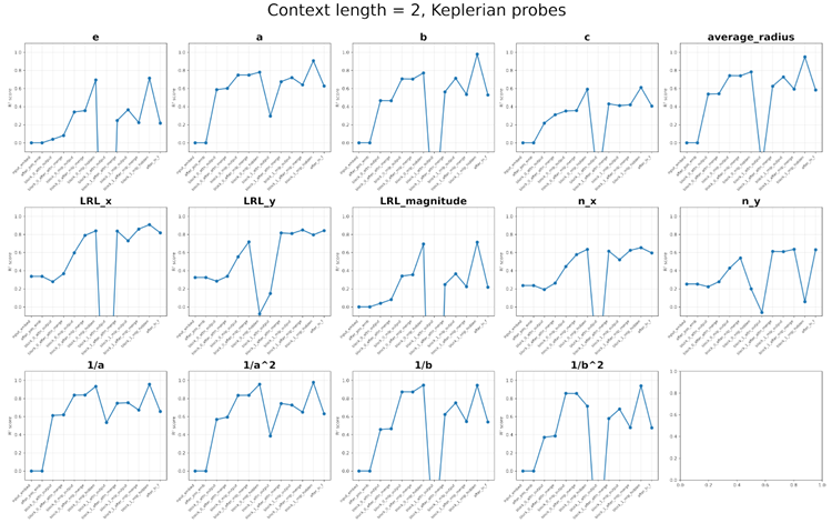
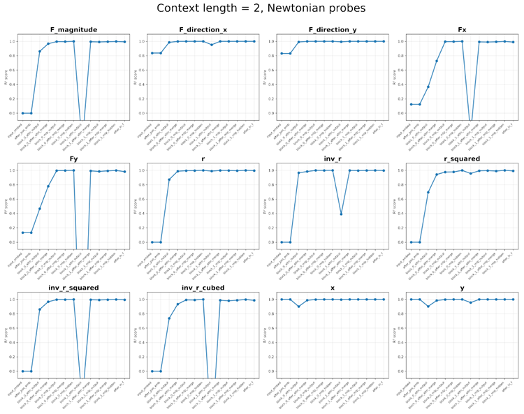
Figure 11. Probing results for context length 2. Top: Probes related to the Keplerian model. Bottom: Probes related to the Newtonian model.
図11. コンテキスト長2のプローブ結果。上:ケプラーモデルに関連するプローブ。下:ニュートンモデルに関連するプローブ。
Keplerian model: semi-major axis length \(a\) (and \(1/a, 1/a^2\)), semi-minor axis length \(b\) (and \(1/b, 1/b^2\)), half focal length \(c = \sqrt{a^2 − b^2}\), ellipticity \(e = c/a\), average radius \(\overline{r} = \sqrt{ab}\), Laplace-Runge-Lenz vector \(\vec{A} = (A_x,A_y)\) and magnitude \(|\vec{A}|\), radial unit vector \(\hat{r}= (n_x,n_y)\).
ケプラーモデル: 長軸の長さ \(a\) (および \(1/a、1/a^2\))、短軸の長さ \(b\) (および \(1/b、1/b^2\))、半焦点距離 \(c = \sqrt{a^2 − b^2}\)、楕円率 \(e = c/a\)、平均半径 \(\overline{r} = \sqrt{ab}\)、ラプラス・ルンゲ・レンツ・ベクトル \(\vec{A} = (A_x、A_y)\) および大きさ \(|\vec{A}|\)、動径単位ベクトル \(\hat{r}= (n_x、n_y)\)。
Newtonian model Gravitational force \(\vec{F} = (F_x,F_y)\) and magnitude \(|\vec{F}|\), force direction \((\hat{F}_x,\hat{F}_y) = \hat{r} = (n_x,n_y)\), position \(\vec{r} = (x,y)\), radius \(r =\sqrt{x^2 + y^2}\) (and \(r^2, 1/r, 1/r^2, 1/r^3\)).
ニュートンモデル 重力 \(\vec{F} = (F_x,F_y)\) と大きさ \(|\vec{F}|\)、力の方向 \((\hat{F}_x,\hat{F}_y) = \hat{r} = (n_x,n_y)\)、位置 \(\vec{r} = (x,y)\)、半径 \(r =\sqrt{x^2 + y^2}\) (および \(r^2, 1/r, 1/r^2, 1/r^3\))。
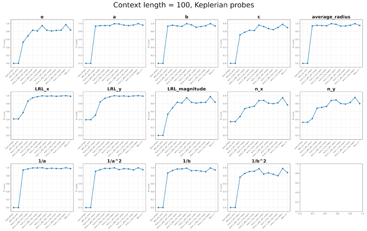
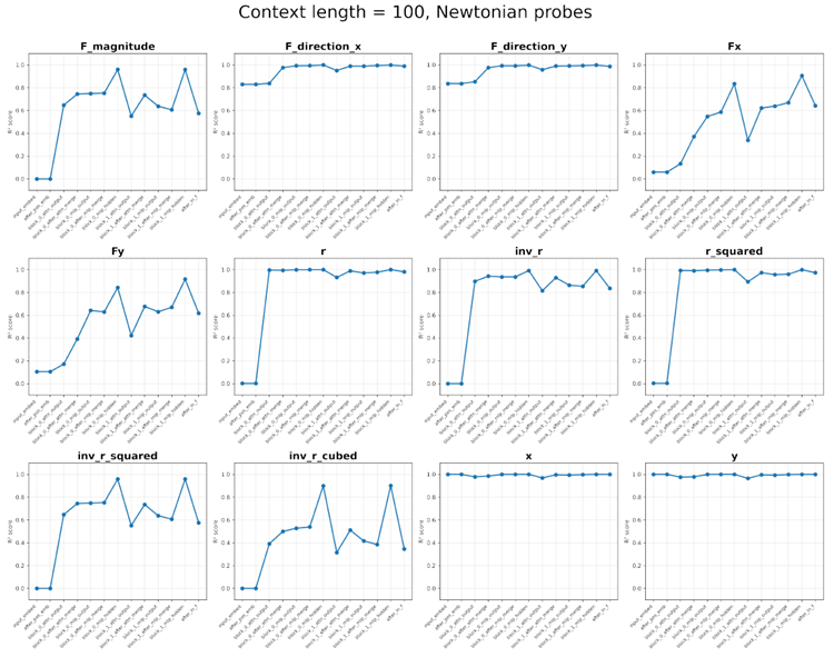
Figure 12. Probing results for context length 100. Top: Probes related to the Keplerian model. Bottom: Probes related to the Newtonian model.
図12. コンテキスト長100のプローブ結果。上:ケプラーモデルに関連するプローブ。下:ニュートンモデルに関連するプローブ。