Blind denoising diffusion models and the blessings of dimensionality

We analyze, theoretically and empirically, the performance of generative diffusion models based on blind denoisers, in which the denoiser is not given the noise amplitude in either the training or sampling processes. Assuming that the data distribution has low intrinsic dimensionality, we prove that blind denoising diffusion models (BDDMs), despite not having access to the noise amplitude, automatically track a particular implicit noise schedule along the reverse process. Our analysis shows that BDDMs can accurately sample from the data distribution in polynomially many steps as a function of the intrinsic dimension. Empirical results corroborate these mathematical findings on both synthetic and image data, demonstrating that the noise variance is accurately estimated from the noisy image. Remarkably, we observe that schedule-free BDDMs produce samples of higher quality compared to their non-blind counterparts. We provide evidence that this performance gain arises because BDDMs correct the mismatch between the true residual noise (of the image) and the noise assumed by the schedule used in non-blind diffusion models.
我々は、ブラインドデノイザーに基づく生成拡散モデルの性能を理論的かつ経験的に分析する。このモデルでは、デノイザーにはトレーニングプロセスでもサンプリングプロセスでもノイズ振幅が与えられない。データ分布の固有次元が低いと仮定し、ブラインドデノイジング拡散モデル (BDDM) はノイズ振幅にアクセスできないにもかかわらず、逆プロセスに沿って特定の暗黙的なノイズスケジュールを自動的に追跡することを証明した。分析によると、BDDM は固有次元の関数として多項式的に多くのステップでデータ分布から正確にサンプリングできる。経験的結果は、合成データと画像データの両方でこれらの数学的発見を裏付け、ノイズ分散がノイズ画像から正確に推定されることを実証した。注目すべきことに、スケジュールフリーの BDDM は、非ブラインドの BDDM と比較して、より高品質のサンプルを生成することがわかった。このパフォーマンスの向上は、BDDM が (画像の) 実際の残差ノイズと非ブラインド拡散モデルで使用されるスケジュールによって想定されるノイズ間の不一致を修正することによって生じるという証拠を示します。

1 Introduction はじめに

Diffusion models have emerged as the dominant methodology for generative modeling and solving inverse problems. In contrast to previous machine learning methods, such as generative adversarial networks (Arjovsky et al., 2017), normalizing flows (Grathwohl et al., 2019), or variational autoencoders (Kingma and Welling, 2013), diffusion models are based on corresponding noise corruption and denoising processes (Sohl-Dickstein et al., 2015; Ho et al., 2020; Song et al., 2021b). In brief, sampling is achieved through discretizations of stochastic differential equations (SDEs) of the form
拡散モデルは、生成モデリングと逆問題解決における主要な手法として登場しました。生成敵対ネットワーク(Arjovsky et al., 2017)、正規化フロー(Grathwohl et al., 2019)、変分オートエンコーダ(Kingma and Welling, 2013)といった従来の機械学習手法とは対照的に、拡散モデルは対応するノイズ破壊とノイズ除去プロセスに基づいています(Sohl-Dickstein et al., 2015; Ho et al., 2020; Song et al., 2021b)。簡単に言うと、サンプリングは、以下の形式の確率微分方程式(SDE)の離散化によって実現されます。 \[ dX_t = \hat{b}_θ(X_t,σ_t)dt + \sqrt{2a_t} dB_t \tag{1} \] where \(\hat{b}_θ: \mathbb{R}^d×\mathbb{R}_+ → \mathbb{R}^d\) is an optimal denoiser, \(dB_t\) is standard Brownian motion, and \((a_t)_{t≥0}\) are diffusion coeficients. The correctness of (1) as a method for sampling from the data distribution holds by design in continuous time, due to the nature of forward and backward diffusion processes (Föllmer, 1985) and the fact that an optimal denoiser computes a scaled version of the score function of the noisy data distribution (Miyasawa, 1961; Efron, 2011; Raphan and Simoncelli, 2011).
ここで、\(\hat{b}_θ: \mathbb{R}^d×\mathbb{R}_+ → \mathbb{R}^d\)は最適なノイズ除去法、\(dB_t\)は標準ブラウン運動、\((a_t)_{t≥0}\)は拡散係数である。データ分布からサンプリングする方法としての(1)の正しさは、順方向拡散過程と逆方向拡散過程の性質(Föllmer, 1985)と、最適なノイズ除去法がノイズを含むデータ分布のスコア関数のスケール版を計算するという事実(Miyasawa, 1961; Efron, 2011; Raphan and Simoncelli, 2011)により、連続時間において意図的に成立する。

In practice, the denoiser is usually implemented as a parametric neural network that takes as input the noisy image (first argument, \(X_σ\)) and the corresponding noise level (second argument, \(σ\)), and is trained to denoise the noisy image. During sampling, (1) is discretized, and a noise schedule is prescribed to provide noise level arguments that ensure that the network follows the appropriate trajectory. Thus, the success of such generative algorithms hinge on training a high-quality denoiser and a noise schedule that that allows \(\hat{b}_θ\) to successfully denoise along the process.
実際には、ノイズ除去装置は通常、パラメトリックニューラルネットワークとして実装されます。このネットワークは、ノイズ画像(第一引数、\(X_σ\))とそれに対応するノイズレベル(第二引数、\(σ\))を入力として受け取り、ノイズ画像のノイズ除去を行うように学習します。サンプリング中、(1)は離散化され、ネットワークが適切な軌跡をたどることを保証するノイズレベル引数を提供するノイズスケジュールが規定されます。したがって、このような生成アルゴリズムの成功は、高品質のノイズ除去装置と、\(\hat{b}_θ\) がプロセス全体にわたってノイズ除去を正常に実行できるノイズスケジュールを学習することにかかっています。

What if the noise level is not passed to the network during training? The resulting blind denoiser, denoted \(\hat{s}_θ: \mathbb{R}^d → \mathbb{R}^d\) (see Section 2.2), must then effectively determine the noise level from the noisy image. Remarkably, blind denoising diffusion models (BDDMs) can be highly effective in sampling from complex distributions and in solving inverse problems (Kadkhodaie and Simoncelli, 2020, 2021). Sampling via BDDMs is based on discretizations of the following dynamics
学習中にノイズレベルがネットワークに渡されない場合はどうなるでしょうか？結果として得られるブラインドデノイザー(\(\hat{s}_θ: \mathbb{R}^d → \mathbb{R}^d\)と表記)(2.2節参照)は、ノイズ画像からノイズレベルを効果的に決定する必要があります。注目すべきことに、ブラインドデノイジング拡散モデル(BDDM)は、複雑な分布からのサンプリングや逆問題の解法において非常に効果的です(Kadkhodaie and Simoncelli, 2020, 2021)。BDDMによるサンプリングは、以下のダイナミクスの離散化に基づいています。 \[ dY_t = \hat{s}_θ(Y_t)dt + \sqrt{2a_t}dB_t \tag{2} \] We emphasize that the drift term (i.e. first term) in (2) is independent of time, suggesting that these dynamics are closer to standard Langevin-type dynamics. But unlike (1), the convergence of this scheme is not clear from the outset. These observations lead us to our first motivating question:
(2) のドリフト項(すなわち第一項)は時間に依存しないことを強調し、この力学が標準的なランジュバン型力学に近いことを示唆する。しかし、(1) とは異なり、このスキームの収束性は最初から明らかではない。これらの観察から、最初の動機となる疑問が浮かび上がる。

Is there a principled explanation for the empirical success of BDDMs?
BDDM の実証的な成功について原理的な説明はあるだろうか?

Beyond theoretical justification, we want to better understand the practical implica-tions of blind denoisers for generative modeling. Indeed, BDDMs have “less information” (namely, they are not given the noise level) than their non-blind counterparts during both training and sampling. Moreover, prior work suggests that noise schedules and time embeddings are not required, minimizing the number of hyperparameters that must be tuned (Sun et al., 2025). Thus, we also ask:
理論的な正当性を超えて、生成モデリングにおけるブラインドデノイザーの実用的な意味合いをより深く理解したいと考えています。実際、BDDMは、訓練時とサンプリング時の両方において、非ブラインドデノイザーよりも「情報量が少ない」(つまり、ノイズレベルが与えられない)のです。さらに、先行研究では、ノイズスケジュールと時間埋め込みは不要であり、調整が必要なハイパーパラメータの数を最小限に抑えられることが示唆されています(Sun et al., 2025)。そこで、私たちは以下の問いかけを提起します。

What are the computational advantages of BDDMs?
BDDM の計算上の利点は何か?

Contributions 貢献

This work provides the first mathematical justification for the success of blind denoising diffusion models.
この研究は、ブラインドノイズ除去拡散モデルの成功を初めて数学的に証明するものです。

Blessings of dimensionality.　Motivated by empirical evidence (Olshausen and Field, 1996; Roweis and Saul, 2000; Chandler and Field, 2007; H´enaff et al., 2014; Pope et al., 2021; Brown et al., 2023), we identify low intrinsic dimensionality of the data distribution \(p_X\) as a natural condition that explains the success of BDDMs. Under this condition, we show that BDDMs provably generate correct samples. Specifically, as a corollary to our main results, we show that the distribution arising from (2), denoted \(p_{alg}\), is close to \(p_X\) if the intrinsic dimension \(k\)is suficiently small, i.e.,
次元性の恩恵　経験的証拠(Olshausen and Field, 1996; Roweis and Saul, 2000; Chandler and Field, 2007; H´enaff et al., 2014; Pope et al., 2021; Brown et al., 2023)に基づき、データ分布 \(p_X\) の低い固有次元性が、BDDM の成功を説明する自然な条件であると特定する。この条件下では、BDDM が正しいサンプルを生成することが証明できることを示す。具体的には、主な結果の帰結として、固有次元 \(k\) が十分に小さい場合、(2) から生じる分布 \(p_{alg}\) は \(p_X\) に近いことを示す。すなわち、

\[ \text{D}(p_X,p_{\text{alg}})\leq ε\quad \text{if }\frac{k^4}{ε^4}\ll d \tag{3} \]

where \(\text{D}(·,·)\) corresponds to a “perceptual” metric between distributions (Corollary 3.10). Building on state-of-the-art works on low-dimensional adaptivity of diffusion models (Huang et al., 2024; Li and Yan, 2024; Potaptchik et al., 2024; Liang et al., 2025; Tang and Yan, 2025), we then proceed to show that the iteration complexity of BDDMs scales as \(k^2/ε^2\).
ここで、\(\text{D}(·,·)\) は分布間の「知覚的」な指標に対応する(系3.10)。拡散モデルの低次元適応性に関する最先端の研究(Huang et al., 2024; Li and Yan, 2024; Potaptchik et al., 2024; Liang et al., 2025; Tang and Yan, 2025)に基づき、BDDMの反復計算量は \(k^2/ε^2\) に比例することを示す。

Our theory also has predictive power: it identifies canonical choices for the diffusion schedule \((a_t)_{t≥0}\), the prior over noise levels during training, and the step size schedule. In particular, our theory suggests that a constant stepsize sufices for sampling, reducing the need to tune noise schedules. In fact, we show that BDDMs track an implicit noise sched-ule, whereby the law of \(Y_t\) in (2) approximates \(p_X∗\mathcal{N}(0,σ_t^2I)\) for a noise schedule given by
我々の理論は予測力も備えている。拡散スケジュール\((a_t)_{t≥0}\)、訓練中のノイズレベルに対する事前分布、そしてステップサイズスケジュールの標準的な選択肢を特定する。特に、我々の理論は、サンプリングには一定のステップサイズで十分であり、ノイズスケジュールを調整する必要性を低減することを示唆している。実際、BDDMは暗黙のノイズスケジュールに従うことを示す。これにより、(2)の\(Y_t\)の法則は、次式で与えられるノイズスケジュールに対して\(p_X∗\mathcal{N}(0,σ_t^2I)\)に近似する。

Key to our approach is the formal introduction of Bayesian statistical estimation of the noise level from a single noisy sample. In some cases, this problem is not solvable (e.g., if pX is Gaussian distributed). However, we show that low intrinsic dimensionality enables consistent estimation. Both of these predictions—namely, that (i) BDDMs track the noise schedule (4) and (ii) the noise level is accurately learned in low intrinsic dimension—are confirmed by our experiments.
私たちのアプローチの鍵となるのは、単一のノイズサンプルからノイズレベルをベイズ統計的に推定することを正式に導入することです。場合によっては、この問題は解けません(例えば、pXがガウス分布に従う場合)。しかし、低い固有次元によって一貫性のある推定が可能になることを示します。これらの予測、すなわち(i) BDDMはノイズスケジュール(4)を追跡し、(ii) 低い固有次元でノイズレベルを正確に学習するという予測は、実験によって確認されました。

Computational benefits of blind denoising.　Turning to our second main ques-tion, we compare the performance of blind and non-blind denoising diffusion models. Starting from the same initial noise sample and injecting the same noise along the trajec-tory, we find that the two diffusion models arrive at dramatically different sample images. We conjecture and verify experimentally that this deviation arises from a subtle but important empirical error in the non-blind setting: along a discretized trajectory in the backward process, the noise prescribed by the explicit schedule and the true noise level on the noisy sample (i.e., \((x_σ,σ) \mapsto \hat{b}_θ(x_σ,σ))\) do not match. In contrast, BDDMs only op-erate on the noisy image as input, and follow an implicit noise schedule naturally inferred from the noisy image, and thus they do not face this mismatch. As a result, we observe that BDDMs produce samples of both higher quality in the constant step size regime.
ブラインドノイズ除去の計算上の利点：2番目の主要な質問に移り、ブラインドおよび非ブラインドノイズ除去拡散モデルのパフォーマンスを比較します。同じ初期ノイズサンプルから開始し、軌跡に沿って同じノイズを注入すると、2つの拡散モデルが劇的に異なるサンプル画像に到達することがわかります。この偏差は、非ブラインド設定における微妙だが重要な経験的誤差から生じると推測し、実験的に検証しました。つまり、逆方向プロセスの離散化軌跡に沿って、明示的なスケジュールで規定されたノイズとノイズサンプルの実際のノイズレベル(つまり、\((x_σ,σ) \mapsto \hat{b}_θ(x_σ,σ))\)は一致しません。対照的に、BDDMはノイズ画像を入力としてのみ操作し、ノイズ画像から自然に推測される暗黙のノイズスケジュールに従うため、この不一致に直面することはありません。その結果、BDDM は一定のステップサイズモードで高品質のサンプルを生成することがわかります。

Related work 関連研究

Blind denoising (diffusion models) ブラインドノイズ除去(拡散モデル)

BDDMs were introduced by Kadkhodaie and Simoncelli (2020, 2021), in which a blind deep neural network denoiser (Zhang et al., 2017) was used to sample from pX in dynam-ics described in (2). Their capabilities for sampling and solving linear inverse problems were demonstrated empirically and their generalization (with respect to training set size) was examined by Kadkhodaie et al. (2024).
BDDMはKadkhodaieとSimoncelli (2020, 2021)によって導入され、ブラインドディープニューラルネットワークデノイザー(Zhang et al., 2017)を用いて、(2)で説明したダイナミクスにおけるpXからのサンプリングが行われた。BDDMのサンプリング能力と線形逆問題の解法は経験的に実証され、その一般化(トレーニングセットのサイズに関して)はKadkhodaie et al. (2024)によって検証された。

Several recent publications (e.g., Li and He, 2025; Wang and Du, 2025) train neural networks to learn dynamics without time inputs. Sun et al. (2025) show that noise conditioning is not required for sampling, and verify this empirically on dynamics which rely on explicit schedules. They also make partial initial progress on a theory for blind denoisers for diffusion models, studying the simple cases where pX is a single Dirac mass or mixture of Dirac masses. We depart from these simple scenarios by showing that blind denoisers can estimate noise levels from images, assuming low intrinsic dimensionality of the underlying data distribution. We provide complete, rigorous derivations (e.g., sampling guarantees) under this assumption, in addition to numerical experiments.
最近のいくつかの出版物(例えば、Li and He、2025年、Wang and Du、2025年)では、ニューラルネットワークを訓練して、時間入力なしでダイナミクスを学習させています。Sun et al.(2025)は、サンプリングにはノイズ調整が必要ないことを示し、明示的なスケジュールに依存するダイナミクスでこれを経験的に検証しています。彼らはまた、拡散モデルのブラインドノイズ除去装置の理論について部分的に初期進展を見せており、pXが単一のディラック質量またはディラック質量の混合である単純なケースを研究しています。私たちはこれらの単純なシナリオから出発して、基礎となるデータ分布の固有次元が低いと仮定して、ブラインドノイズ除去装置が画像からノイズレベルを推定できることを示します。私たちは数値実験に加えて、この仮定の下で完全で厳密な導出(例えば、サンプリング保証)を提供します。

Sample complexity of diffusion models 拡散モデルのサンプル複雑性

Chen et al. (2023) and Lee et al. (2023) were among the first to provide a discretization analysis of (non-blind) denoising diffusion models specialized to the SDE case. They showed that suficiently well-approximated score functions (equivalently, our assumption (A3) below) can sample from a target distribution in polynomial time. A flurry of works swiftly followed, hoping to improve the bounds initially published in these works. For example, Benton et al. (2024) and Conforti et al. (2025) both proposed using time-dependent noise schedules to obtain a tighter dimension dependence. A subsequent line of work has shown that sampling guarantees for non-blind denoising diffusion models scales with the intrinsic dimensionality of the data, not the ambient dimension, corresponding to our (A2) (Huang et al., 2024; Li and Yan, 2024; Potaptchik et al., 2024). Fundamentally our results are incomparable as these works all study non-blind denoising diffusion models.
Chen et al. (2023) と Lee et al. (2023) は、SDE の場合に特化した(非ブラインド)ノイズ除去拡散モデルの離散化解析を初めて提供した研究の一つである。彼らは、十分に近似されたスコア関数(つまり、以下の我々の仮定 (A3) と同等)が、多項式時間でターゲット分布からサンプリングできることを示した。その後、これらの研究で最初に発表された境界を改善しようとする多くの研究が急速に続いた。例えば、Benton et al. (2024) と Conforti et al. (2025) はどちらも、より厳密な次元依存性を得るために時間依存ノイズスケジュールを用いることを提案した。その後の研究により、非ブラインドノイズ除去拡散モデルのサンプリング保証は、環境次元ではなくデータの固有次元に比例することが示されており、これは我々の研究(A2)に相当します(Huang et al., 2024; Li and Yan, 2024; Potaptchik et al., 2024)。これらの研究はすべて非ブラインドノイズ除去拡散モデルを研究しているため、基本的に我々の結果は比較できません。

Notation 表記法

We denote the centered Gaussian with variance \(σ^2 \gt 0\) as \(γ_{σ^2} = \mathcal{N}(0,σ^2I)\). Throughout, we denote the data distribution as \(p_X\), and the noisy data distribution(s) as \(p_σ = p_X ∗γ_{σ^2}\). We let \(dB_t\) denote standard Brownian motion. We use \(a ≲ b \)(resp. \(a ≳ b\)) to mean that there exists a constant \(C\) such that \(a ≤ Cb\) (resp. a constant \(c\) such that \(a ≥ cb\)). If both \(a ≲ b\) and \(b ≲ a\), then we write \(a ≍ b\). We use, for example, \(a ≲_{\log} b\) to ignore logarithmic factors (in \(b\)). Finally, a ball of radius \(R > 0\) centered at \(a ∈ \mathbb{R}^d\) is denoted by \(B(a,R)\).
分散 \(σ^2 \gt 0\) の中心ガウス分布を \(γ_{σ^2} = \mathcal{N}(0,σ^2I)\) と表記する。全体を通して、データ分布を \(p_X\)、ノイズを含むデータ分布を \(p_σ = p_X ∗γ_{σ^2}\) と表記する。\(dB_t\) は標準ブラウン運動を表す。\(a ≲ b \)(あるいは \(a ≳ b\)) は、\(a ≤ Cb\) となる定数 \(C\) が存在すること (あるいは \(a ≥ cb\) となる定数 \(c\) が存在することを意味する)。 \(a ≲ b\) かつ \(b ≲ a\) の両方が成り立つ場合、\(a ≍ b\) と書きます。例えば、\(b\) 内の対数係数を無視するには、\(a ≲_{\log} b\) と書きます。最後に、\(a ∈ \mathbb{R}^d\) を中心とする半径 \(R > 0\) の球体は \(B(a,R)\) と表されます。

2 Preliminaries 準備

2.1 Primer on variance exploding diffusion models 分散発散拡散モデルの入門

We first briefly review background material on variance-exploding (VE) diffusion models.
まず、分散発散 (VE) 拡散モデルに関する背景資料を簡単に確認します。

For a fixed terminal time \(T \gt 0\) and diffusion schedule \((a_t)_{t∈[0,T]}\) with \(a_t \geq 0\), consider the forward noising SDE
固定の終端時刻\(T \gt 0\)と拡散スケジュール\((a_t)_{t∈[0,T]}\)、\(a_t \geq 0\)の場合、順方向ノイズSDEを考える。 \[ dX_t = \sqrt{2a_t}dB_t \] where \(X_0 \sim p_X\). Then, \(\text{Law}(X_t) = p_{σ_t} = p_X ∗ γ_{σ_t^2}\), where \(σ_t^2 = 2\int_0^t a_s ds\). Following the theory of SDEs (Föllmer, 1985), the time-reversed process can be written as
ここで\(X_0 \sim p_X\)である。そして\(\text{Law}(X_t) = p_{σ_t} = p_X ∗ γ_{σ_t^2}\)であり、\(σ_t^2 = 2\int_0^t a_s ds\)である。SDE理論(Föllmer, 1985)に従うと、時間反転過程は次のように表される。 \[ dX_t^← = −a_t∇\log p_{σ_{T−t}}(X_t^←)dt +\sqrt{2_at}dB_t \] where now \(X_t^←:= X_{T−t} \sim p_{σ_{T−t}}\).
ここで\(X_t^←:= X_{T−t} \sim p_{σ_{T−t}}\)です。

The reverse process above is driven by ∇logpσt, known as the score function. A standard calculation known as Tweedie’s formula (Miyasawa, 1961; Efron, 2011; Raphan and Simoncelli, 2011) relates the score to the posterior mean:
上記の逆のプロセスは、スコア関数として知られる∇logpσtによって駆動されます。Tweedieの式(Miyasawa, 1961; Efron, 2011; Raphan and Simoncelli, 2011)として知られる標準的な計算法は、スコアと事後平均を関連付けます。 \[ s_{σ_t}^\star(y):= σ_t^2∇\log p_{σ_t}(y) = \mathbb{E}[X|Y= y]− y \tag{5} \] where we take the conditional expectation of \(X\) given \(Y\) in the model \(X \sim p_X, Y \sim \mathcal{N}(X,σ_t^2I)\). In other words, the score function of \(p_Y\) is proportional to the difference between the denoiser (the posterior mean \(\mathbb{E}[X|Y = y]\)), and the noisy sample \(y\).
ここで、モデル\(X \sim p_X, Y \sim \mathcal{N}(X,σ_t^2I)\)において、\(X\)が与えられた場合の\(Y\)の条件付き期待値を取ります。言い換えれば、\(p_Y\)のスコア関数は、ノイズ除去サンプル(事後平均\(\mathbb{E}[X|Y = y]\))とノイズサンプル\(y\)の差に比例します。

2.2 Training and sampling with blind denoisers ブラインドデノイザーによるトレーニングとサンプリング

Unlike standard denoisers in the diffusion model literature, blind denoiser are not given the noise level during training. Letting \(f_θ: \mathbb{R}^d → \mathbb{R}^d\) denote a neural network, a blind denoiser is trained using the following objective:
拡散モデルの文献で紹介されている標準的なノイズ除去装置とは異なり、ブラインドノイズ除去装置は学習中にノイズレベルを与えられません。\(f_θ: \mathbb{R}^d → \mathbb{R}^d\) をニューラルネットワークとすると、ブラインドノイズ除去装置は以下の目的関数を用いて学習されます。 \[ \hat{f}_θ = \text{arg}\min\limits_θ\frac{1}{n}\sum_{i=1}^n\underset{\substack{σ\sim Θ \\ z\sim γ}}{\mathbb{E}}||x_i − f_θ(x_i + σz)||^2\tag{6} \] where \(\{x_i\}_{i=1}^n \sim p_X\) are the clean training samples, \(γ\) is the standard Gaussian in \(\mathbb{R}^d\), and \(Θ\) is a prior distribution over noise levels in the range \([σ_T ,σ_0]\), with \(0 \lt σ_T \lt σ_0 \lt +∞\). (Since we are interested in the reverse process, \(σ_0\) is the largest noise level, and \(σ_T\) is the smallest.) In practice, we minimize (6) using (batch) stochastic gradient descent, see Algorithm 1 for pseudocode.
ここで、\(\{x_i\}_{i=1}^n \sim p_X\)はクリーンなトレーニングサンプル、\(γ\)は\(\mathbb{R}^d\)の標準ガウス分布、\(Θ\)は\([σ_T ,σ_0]\)の範囲のノイズレベル(\(0 \lt σ_T \lt σ_0 \lt +∞\) の事前分布です。(逆のプロセスに関心があるため、\(σ_0\) が最大ノイズレベル、\(σ_T\) が最小ノイズレベルとなります。)実際には、(バッチ)確率的勾配降下法を使用して(6)を最小化します。擬似コードについてはアルゴリズム1を参照してください。

To sample, we initialize \(Y_0 ∼ \mathcal{N}(0,σ^2I)\) and consider various discretizations of
サンプリングするために、\(Y_0 ∼ \mathcal{N}(0,σ^2I)\)を初期化し、 \[ dY_t = (\hat{f}_θ(Y_t) − Y_t)dt + \sqrt{2a_t}dB_t \tag{7} \] see Algorithm 2. For example, a standard Euler discretization results in
アルゴリズム2を参照。例えば、標準的なオイラー離散化では、 \[ Y_{(k+1)h} = Y_{kh} + h(\hat{f}_θ(Y_{kh}) − Y_{kh}) + \mathcal{N}(0,2a_thI) \] where \(h > 0\) is a constant step size, and \((a_t)_{t≥0}\) is a predetermined diffusion coeficient schedule. We additionally discuss the exponential (Euler) integrator in Appendix C.1, as it plays a role in our analysis.
ここで、\(h > 0\) は定数ステップサイズ、\((a_t)_{t≥0}\) は予め定められた拡散係数スケジュールです。本解析において重要な役割を果たす指数積分(オイラー積分)については、付録C.1でさらに説明します。

3 Theoretical contributions 理論的貢献

This section contains our theoretical contributions, which rigorously justify the use of BDDMs as generative models. All proofs are provided in the appendix.
このセクションでは、BDDMを生成モデルとして使用することを厳密に正当化する理論的貢献について説明します。すべての証明は付録に記載されています。

3.1 The optimal blind denoiser 最適なブラインドノイズ除去装置

The first step is to understand the population minimizer of the blind denoising problem (6): Given infinite data and perfect optimization, what is (6) learning? Since the noise level is not known, it should be treated as a random variable as opposed to a known parameter. From a Bayesian perspective, the optimal solution then comes from marginalizing over this random variable. The following theorem makes this precise and indicates that the optimal blind denoiser can be expressed as a conditional average of score functions.
最初のステップは、ブラインドノイズ除去問題(6)の母集団最小化元を理解することです。無限データと完全最適化が与えられた場合、(6)の学習とは一体何でしょうか？ノイズレベルは未知であるため、既知のパラメータではなく、ランダム変数として扱う必要があります。ベイズ理論の観点から見ると、最適解はこのランダム変数を周辺化することで得られます。次の定理はこれを明確化し、最適なブラインドノイズ除去問題がスコア関数の条件付き平均として表現できることを示しています。

Proposition 3.1: Optimal blind denoiser 命題3.1: 最適なブラインドノイズ除去装置

The population minimizer of (6) is
(６)の母集団最小化元は \[ f^⋆: y \mapsto y +\int σ^2∇\log p_σ(y)dµ(σ|y) \] where \(p_σ:= p_X ∗ \mathcal{N}(0,σ^2I)\), and
ここで \(p_σ:= p_X ∗ \mathcal{N}(0,σ^2I)\)、そして \[ µ(σ|y) ∝ \frac{Θ(σ)}{σ^d} \mathbb{E}_{X\sim p_X}\left[ \exp\left(−\frac{σ^{−2}}{2}||X − y||^2\right)\right] \tag{8} \]

We can thus- express the optimal blind score function as an integral over the mixture, i.e.,
したがって、最適なブラインドスコア関数は混合の積分として表現できる。すなわち、 \[ s^⋆(y):= f^⋆(y) − y = \int σ^2∇\log p_σ(y)dµ(σ|y) \tag{9} \]

3.2 Derivation of the implicit noise schedule 暗黙のノイズスケジュールの導出

We now examine the dynamics arising from the optimal blind score function (9). To start, we consider the continuous-time analogue of the dynamics suggested by the algorithm of Kadkhodaie and Simoncelli (2020) with a perfectly trained denoiser, which are given by
最適なブラインドスコア関数(9)から生じるダイナミクスを考察する。まず、KadkhodaieとSimoncelli (2020)のアルゴリズムで提案されたダイナミクスの連続時間アナログを、完全に学習されたノイズ除去器を用いて考察する。これは次のように与えられる。 \[ dX_t^⋆ = s^⋆(X_t^⋆)dt + \sqrt{2a_t}dB_t \tag{10} \] where we initialize with \(X_0^\star \sim \mathcal{N}(0,σ_0^2I)\).
ここで\(X_0^\star \sim \mathcal{N}(0,σ_0^2I)\)で初期化します。

We consider the following ansatz: for all \(t, X_t^\star\) is approximately distributed as \(p_{σ_t}\), for some denoising schedule \((σ_t)_{t≥0}\) (to be derived). Further, let us suppose that when y = Xt , then the conditional distribution \(µ(σ|X_t^\star)\) in (8) concentrates on the true noise level \(σ_t\). By (9), this suggests considering the following process in which we replace the conditional average over noise levels with \(σ_t\):
以下の仮定を考える：すべての\(t, X_t^\star\)は、\(p_{σ_t}\)のように近似的に分布する。あるノイズ除去スケジュール\((σ_t)_{t≥0}\)（導出予定）に対しても同様である。さらに、y = Xtのとき、(8)式の条件付き分布\(µ(σ|X_t^\star)\)が真のノイズレベル\(σ_t\)に集中すると仮定する。(9)式から、これはノイズレベルの条件付き平均を\(σ_t\)に置き換える以下のプロセスを考慮することを示唆している。 \[ dX_t = s_{σ_t}^\star (X_t)dt + \sqrt{2a_t} dB_t := (σ_t^2∇\log p_{σ_t}(X_t))dt +\sqrt{2a_t} dB_t \tag{11} \] However, along (11), the evolution of the density is given by SDE theory, in particular by the Fokker–Planck equation. In order to be consistent with the ansatz \(\text{Law}(X_t)\approx p_{σ_t}\), this implies the following ODE for \(σ_t\) (see Appendix A.2):
しかしながら、(11)式に沿って、密度の発展はSDE理論、特にフォッカー・プランク方程式によって与えられます。\(\text{Law}(X_t)\approx p_{σ_t}\)という仮定と整合させるために、\(σ_t\)について以下の常微分方程式が成り立ちます（付録A.2を参照）。 \[ σ_t\dot{σ}_t = −σ_t^2 + a_t \tag{12} \] Solving this ODE, we arrive at the following result.
この ODE を解くと、次の結果が得られます。

Proposition 3.2: Implicit noise schedule 命題3.2: 暗黙のノイズスケジュール

The ideal dynamics (11) satisfies \(\text{Law}(X_t) = p_{σ_t}\) for all \(t ≥ 0\), provided that
理想的な力学(11)は、すべての\(t ≥ 0\)に対して\(\text{Law}(X_t) = p_{σ_t}\)を満たす。ただし、 \[ σ_t^2 = σ_0^2e^{−2t} + 2 \int_0^t a_se^{−2(t−s)} ds \]

We record two properties of this noise schedule.
このノイズスケジュールの 2 つの特性を記録します。

Lemma 3.3.　If \(t \mapsto a_t\) is decreasing and \(a_0 ≤ σ_0^2\), then \(t \mapsto σ_t\) is decreasing.
補題3.3　\(t \mapsto a_t\) が減少傾向にあり、\(a_0 ≤ σ_0^2\) であれば、\(t \mapsto σ_t\) は減少傾向にある。

Lemma 3.4.　If \(t \mapsto a_t\) is decreasing and \(a_t → 0\) as \(t → ∞\), then \(σ_t → 0\) as well.
補題3.4　\(t \mapsto a_t\)が減少し、\(t → ∞\)のときに\(a_t → 0\)となる場合、\(σ_t → 0\)も同様に減少する。

Henceforth, we assume that the conditions of Lemma 3.4 hold. discussion suggests that if \(µ(·|X_t)\) concentrates around \(σ_t\) such that
これから、補題3.4の条件が成り立つと仮定する。議論によれば、\(µ(·|X_t)\)が\(σ_t\)の周囲に集中し、 \[ \int σ^2∇\log p_σ(y)dµ(σ|X_t) \approx σ_t^2∇\log p_{σ_t}(X_t) \tag{13} \] and if \(a_t → 0\), then heuristically we expect \(\text{Law}(X_t^\star) \approx \text{Law}(X_t) → p_X\) as \(t → ∞\).
そして\(a_t → 0\)の場合、経験的に\(t → ∞\)のときに\(\text{Law}(X_t^\star) \approx \text{Law}(X_t) → p_X\)が期待されます。

We stress that at no point during the sampling process will the blind denoiser be given information about the schedule \(σ_t\). Instead, it must adapt to this schedule automatically by estimating \(σ_t\) from the current input \(Y_t\). In other words, if \(µ(σ|X_t)\) concentrates, the \(σ_t\) for which \(p_{σ_t} = p_X ∗ \mathcal{N}(0,σ_t^2I)\) can be inferred from input \(Y_t\). This is because \(p_σ(Y_t)\) would be negligible for all \(σ\) but a small set around \(σ_t\). As a result, the ideal dynamics in the backward process should follow the true schedule \(σ_t\) given above.
サンプリング処理のどの時点でも、ブラインドデノイザーにはスケジュール \(σ_t\) に関する情報は与えられないことを強調しておきます。代わりに、ブラインドデノイザーは、現在の入力 \(Y_t\) から \(σ_t\) を推定することで、このスケジュールに自動的に適応する必要があります。言い換えれば、\(µ(σ|X_t)\) が集中する場合、\(p_{σ_t} = p_X ∗ \mathcal{N}(0,σ_t^2I)\) となる \(σ_t\) は入力 \(Y_t\) から推測できます。これは、\(p_σ(Y_t)\) が \(σ_t\) の近傍の小さな集合を除くすべての \(σ\) に対して無視できるためです。結果として、逆方向処理における理想的なダイナミクスは、上記に示した真のスケジュール \(σ_t\) に従うはずです。

3.3 Error bound without discretization 離散化なしの誤差境界

Suppose now that we have an empirical minimizer \(\hat{f}_θ\) that will act as the blind denoiser, and let \(\hat{p}_t := \text{Law}(Y_t)\) along the trained dynamics (7). For now, we omit discretization error, deferring this discussion to Section 3.5. Our goal is to bound the KL divergence between \(\hat{p}_T\), the distribution corresponding to our algorithm at time \(T\), and the target distribution with some small additional noise \(p_{σ_T} = p_X ∗ \mathcal{N}(0,σ_T^2 I)\).
ここで、ブラインドデノイザーとして機能する経験的最小化関数 \(\hat{f}_θ\) があり、訓練されたダイナミクス (7) に沿って \(\hat{p}_t := \text{Law}(Y_t)\) と仮定する。ここでは離散化誤差については省略し、この議論は3.5節に委ねる。目標は、時刻 \(T\) におけるアルゴリズムに対応する分布 \(\hat{p}_T\) と、小さな追加ノイズ \(p_{σ_T} = p_X ∗ \mathcal{N}(0,σ_T^2 I)\) を含む目標分布との間のKLダイバージェンスを制限することである。

By a standard application of Girsanov’s theorem, we can decompose this error into the following terms using the triangle inequality:
ギルサノフの定理を標準的に適用すると、三角不等式を使用してこの誤差を次の項に分解できます。 \[ KL(p_{σ_T}||\hat{p}_T) ≲ KL(p_{σ_0}||\hat{p}_0) + \int_0^T\frac{1}{a_t}\left(||\hat{f}_θ − f^⋆||_{L^2(p_{σ_t})}+||s_{σ_t} − s^⋆||_{L^2(p_{σ_t})}\right) dt \tag{14} \] The first term on the right-hand side corresponds to the initialization error. The second term measures how close the trained denoiser is to the optimal one (the “score error”). Finally, the third term is related to the error in the approximation (13), i.e., the error in estimating the noise level. This last term is the primary novelty over prior work on diffusion models, so we focus our attention on it.
右辺の第1項は初期化誤差に対応する。第2項は、学習済みノイズ除去器が最適なノイズ除去器にどれだけ近いか（「スコア誤差」）を表す。最後に、第3項は近似式(13)の誤差、すなわちノイズレベルの推定誤差に関係する。この最後の項は、拡散モデルに関する先行研究に対する主要な新規性であるため、本研究ではこれに焦点を当てる。

Before stating our main results, we require the following assumptions and definitions. The support of our data distribution will be denoted by \(\mathcal{X}:= supp(p_X)\), and we let \(k\) denote the “intrinsic dimension” of \(p_X\), defined as follows.
主要な結果を述べる前に、以下の仮定と定義が必要である。データ分布のサポートは\(\mathcal{X}:= supp(p_X)\)と表され、\(k\)は\(p_X\)の「固有次元」を表し、以下のように定義される。

Definition 3.5 (Intrinsic dimension).　If \(p_X\) has support \(\mathcal{X}\), we define the intrinsic dimension of \(p_X\) at scale \(r_0\) to be \(k := 1+\log N_{\mathcal{X}}(r_0)\), where \(N_{\mathcal{X}}(r_0)\) denotes the minimal number of balls of radius \(r_0\) needed to cover \(\mathcal{X}\).
定義 3.5 (固有次元). \(p_X\) がサポート \(\mathcal{X}\) を持つ場合、スケール \(r_0\) における \(p_X\) の固有次元を \(k := 1+\log N_{\mathcal{X}}(r_0)\) と定義します。ここで、\(N_{\mathcal{X}}(r_0)\) は \(\mathcal{X}\) を覆うのに必要な半径 \(r_0\) の球の最小数を表します。

For example, if \(\mathcal{X}\) is a \(k\)-dimensional subspace and \(\mathcal{X}\) has diameter \(R\), then \(k ≍ k \log(R/r_0)\). But the intrinsic dimension captures a broader range of situations such as manifold structure, or when \(\mathcal{X}\) is actually full-dimensional but resembles a \(k\)-dimensional manifold at scale \(r_0\). Our proofs require \(r_0 = σ_T^2/(σ_0\sqrt{d})\) as the choice of scale.
例えば、\(\mathcal{X}\) が \(k\) 次元部分空間で、\(\mathcal{X}\) の直径が \(R\) である場合、\(k ≍ k \log(R/r_0)\) となります。しかし、固有次元は、多様体構造や、\(\mathcal{X}\) が実際にはフル次元であるものの、スケール \(r_0\) において \(k\) 次元多様体に類似している場合など、より広範な状況を捉えます。証明では、スケールの選択として \(r_0 = σ_T^2/(σ_0\sqrt{d})\) を要求します。

Our assumptions are the following.
私たちの仮定は次のとおりです。

(A1) \(\mathcal{X} ⊂ B(0,R)\) for some \(R > 0\).
　　何らかの\(R > 0\)に対して\(\mathcal{X} ⊂ B(0,R)\)が成り立つ。

(A2) \(p_X\) has low intrinsic dimensionality, with \(k^2 ≪_{log} d\).
　　\(p_X\) は、\(k^2 ≪_{log} d\) と、固有次元が低い。

(A3) For \(ε_{BD} \gt 0\), \(\int_0^T a_t^{−1}||\hat{f}_θ − f^⋆||_{L^2(p_{σ_t})} dt ≤ ε_{BD}^2\).
　　\(ε_{BD} \gt 0\) に対して、\(\int_0^T a_t^{−1}||\hat{f}_θ − f^⋆||_{L^2(p_{σ_t})} dt ≤ ε_{BD}^2\) です。

Note that (A1), (A2), and (A3) are relatively mild. In particular, (A2) is in-spired from empirical observations (Olshausen and Field, 1996; Roweis and Saul, 2000; Chandler and Field, 2007; H´enaff et al., 2014; Pope et al., 2021; Brown et al., 2023) and has been leveraged in several other works on sampling via diffusion models (Li and Yan, 2024; Pooladian and Niles-Weed, 2025; Liang et al., 2025). (A3) is analogous to the standard assumption that the score functions are accurately learned in L2. In its current form, it is somewhat obscure; we provide further discussion in Section 3.7 when we specialize to specific noise schedules.
(A1)、(A2)、(A3) は比較的軽微なことに留意してください。特に、(A2) は経験的観察 (Olshausen and Field, 1996; Roweis and Saul, 2000; Chandler and Field, 2007; H´enaff et al., 2014; Pope et al., 2021; Brown et al., 2023) に着想を得たものであり、拡散モデルによるサンプリングに関する他のいくつかの研究 (Li and Yan, 2024; Pooladian and Niles-Weed, 2025; Liang et al., 2025) でも活用されています。(A3) は、スコア関数が L2 で正確に学習されるという標準的な仮定に類似しています。現状ではややわかりにくいため、特定のノイズスケジュールに特化して、セクション 3.7 でさらに詳しく説明します。

We are now in a position to state our first main result.
私たちは今、最初の主要な結果を述べる立場にあります。

Theorem 3.6: Error bound without discretization 定理3.6: 離散化なしの誤差限界

Under (A1)–(A3), the KL divergence between the (reverse) processes (7) and (11) is bounded by
(A1)-(A3)の下では、(逆)過程(7)と(11)の間のKLダイバージェンスは、 \[ KL(p_{σ_T}||\hat{p}_T) ≲_{\log}\frac{R^2}{σ_0^2}+ ε_{BD}^2 +\frac{(R^2 + k)k^2}{d}A_T \] where \(A_T = \int_0^T (a_t)^{−1} dt\).

The first term (initialization error) is made small with a suitably large choice of \(σ_0^2\), and the second term (the “score error”) is small if the training is successful. The third term, which scales with \(k\), is discussed next.
最初の項（初期化誤差）は、\(σ_0^2\)を適切に大きくすることで小さくなり、2番目の項（「スコア誤差」）は、学習が成功すれば小さくなります。\(k\)に比例する3番目の項については、次に説明します。

3.4 Interpretation as a Bayesian problem ベイズ問題としての解釈

We now provide an overview of our proof with rigorous details deferred to the ap- pendix. As the first two terms in Theorem 3.6 are standard, we focus on the novel term \(\int_0^T a_t^{−1}||s_{σ_t} − s^⋆||_{L^2(p_{σ_t})}^2 dt\) which captures the error in estimating the noise level.
ここでは証明の概要を示し、厳密な詳細は付録に譲る。定理3.6の最初の2項は標準的な項であるため、ここではノイズレベルの推定における誤差を表す新しい項\(\int_0^T a_t^{−1}||s_{σ_t} − s^⋆||_{L^2(p_{σ_t})}^2 dt\)に焦点を当てる。

Note that for \(X_t ∼ p_{σ_t}\)
\(X_t ∼ p_{σ_t}\) の場合に注意する。 \[ \begin{align} \left|\left|(s_{σ_t}^\star − s^⋆)(X_t)\right|\right|^2 &= \left|\left|\int σ^2∇\log p_σ(X_t)d(δ_{σ_t} − µ(σ|X_t))\right|\right|^2 \\ \\ &= \left|\left| \int \int_σ^{σ_t} ∂_ω(ω^2∇\log p_ω(X_t))dω dµ(σ|X_t)\right|\right|^2 \end{align} \] where we used the fundamental theorem of calculus in the last line. A simple calculation shows that
最後の行では微積分学の基本定理を用いています。簡単な計算で次のことがわかります。 \[ ∂_ω(ω^2∇\log p_ω(y)) = ω^{−3}Cov_{q_ω}(X,||X − Y||^2|Y = y) \] where under \(q_ω\) we have \(X ∼ p_X, Y ∼ \mathcal{N}(X,ω^2I)\). We show in Proposition B.1 that the conditional covariance is bounded in terms of the intrinsic dimension k, essentially leading to a bound on the above term of order
ここで\(q_ω\)のもとで\(X ∼ p_X, Y ∼ \mathcal{N}(X,ω^2I)\)が成り立つ。命題B.1では、条件付き共分散は固有次元kに関して有界であり、本質的に上記の項の順序の上限につながることを示す。 \[ (R^2 + k)k^2 σ_t^4 \int |σ_t^{−2} − σ^{−2}|^2 dµ(σ|X_t) \] The remainder of the analysis is a frequentist analysis of a Bayesian method: We have an observation \(X_t ∼ p_{σ_t}\), where \(σ_t\) is the “ground truth” noise level. We ask whether the posterior distribution on the noise level \(µ(·|X_t)\) concentrates on \(σ_t\) given a single sample. For interpretability, we focus on the class of power law priors \(Θ(σ) ∝ σ^{α−3}\) on \([σ_T ,σ_0]\) for \(α ∈ \mathbb{R}\), and we use the following change of variables.
分析の残りの部分は、ベイズ法の頻度主義的分析である。観測値 \(X_t ∼ p_{σ_t}\) があり、\(σ_t\) は「真の」ノイズレベルである。単一サンプルを与えられた場合、ノイズレベル \(µ(·|X_t)\) の事後分布が \(σ_t\) に集中するかどうかを問う。解釈可能性を高めるため、\(α ∈ \mathbb{R}\) に対して \([σ_T ,σ_0]\) 上のべき乗法則事前分布 \(Θ(σ) ∝ σ^{α−3}\) のクラスに注目し、以下の変数変換を用いる。

Lemma 3.7.　If \(σ ∼ µ(·|y)\) in (8), then \(λ := σ^{−2}\) is distributed according to:
補題3.7　(8)において\(σ ∼ µ(·|y)\)が成り立つ場合、\(λ := σ^{−2}\)は次式に従って分布する: \[ ν(λ|y) ∝ λ^{(d−α)/2} \mathbb{E}_{X∼p_X}\left[\exp\left(−\frac{λ}{2}||X − y||^2\right)\right] \tag{15} \] Writing \(ℓ(λ|y) := −\log ν(λ|y)\), then
\(ℓ(λ|y) := −\log ν(λ|y)\) と書くと、 \[ \begin{align} ℓ^\prime(λ|y) &= −\frac{d-α}{2λ}+\frac{1}{2}\mathbb{E}_{q_λ}[||X − Y||^2|Y = y] \\ ℓ^{\prime\prime}(λ|y) &= \frac{d-α}{2λ^2}−\frac{1}{4} Var_{q_λ}(||X − Y||^2|Y = y) \end{align} \] where, in an abuse of notation, we use qλ to denote the joint distribution for which \(X ∼ p_X, Y ∼ \mathcal{N}(X,λ^{−1}I)\).
ここで、表記法の乱用として、qλを\(X ∼ p_X, Y ∼ \mathcal{N}(X,λ^{−1}I)\)となる結合分布を表すために使用します。

Notice that there is no reason for \(ℓ^{\prime\prime}(·|y)\) to always be convex, given the presence of a negative sign on the second term. However, our low intrinsic dimensionality assumption (A2) nevertheless allows us to show that the noise variance posterior concentrates on the ground truth signal \(λ_t := σ_t^{−2}\).
第2項に負の符号が存在することを考慮すると、\(ℓ^{\prime\prime}(·|y)\)が常に凸になる理由はないことに注意する。しかしながら、我々の低次元性仮定(A2)により、ノイズ分散事後分布が真の信号\(λ_t := σ_t^{−2}\)に集中することを示すことができる。

Proposition 3.8: Estimating the noise level 命題3.8: ノイズレベルの推定

Under (A1)–(A2), for \(X_t ∼ p_{σ_t}, λ ∼ ν(·|X_t)\),
(A1)-(A2) のもとで、\(X_t ∼ p_{σ_t}, λ ∼ ν(·|X_t)\) に対して、 \[ \mathbb{E}|λ − λ_t|^2 ≲_{\log} λ_t^2(d^{−1}+ k^2d^{−2}) \]

Combining these the ingredients yields the claimed bound on the noise level term.
これらの要素を組み合わせると、ノイズレベル項の要求された境界が得られます。

3.5 Discretization, noise, and step size schedules 離散化、ノイズ、ステップサイズスケジュール

A family of convenient diffusion schedules.　Although our results apply to general choices of \((a_t)_{t≥0}\), for the sake of exposition we specialize to a particular con-venient family in order to state our next results in a more interpretable form. Namely, if we take \(a_t = aσ_t^2\) for some \(a ∈ (0,1)\), then the ODE (12) becomes particularly easy to solve: \(σ_t = σ_0e^{−(1−a)t}\). We henceforth fix this particular schedule.
便利な拡散スケジュールの族　我々の結果は\((a_t)_{t≥0}\)の一般的な選択に当てはまるが、説明のために、次の結果をより解釈しやすい形で述べるために、特定の便利な族に特化する。すなわち、ある\(a ∈ (0,1)\)に対して\(a_t = aσ_t^2\)とすると、常微分方程式(12)は特に簡単に解ける：\(σ_t = σ_0e^{−(1−a)t}\)。以下、この特定のスケジュールを固定する。

Discretization error.　If the SDE (7) is discretized, then in addition to the error terms present in Theorem 3.6, we will also incur a discretization error. In order to establish an iteration bound which also scales with the intrinsic dimension, we consider the exponential Euler integrator (see Appendix C.1). With this choice, the discretization error takes the following form: Writing \(t_− := ⌊t/h⌋h\) where \(h\) is the step size, thus \(N = T/h\) is the total number of iterations,
離散化誤差 SDE (7) を離散化すると、定理 3.6 で示されている誤差項に加えて、離散化誤差も発生します。固有次元に比例する反復境界を確立するために、指数オイラー積分器 (付録 C.1 参照) を検討します。この選択により、離散化誤差は次のようになります。\(t_− := ⌊t/h⌋h\) と書きます。ここで \(h\) はステップサイズ、したがって \(N = T/h\) は反復回数です。 \[ \text{Disc}(h) = \int_0^T a_t^{−1} \mathbb{E}||f_{σ_{t_{-}}}^⋆(X_{t_{-}}) − f_{σ_t}^⋆(X_t)||^2 dt \] (Indeed \(\text{Disc}(h)\) arises from (14) if we also incorporate discretization error.) Here, \(f_σ^\star\) denotes the Bayes denoiser when the noise level is known: \(f_σ^\star(y):= \mathbb{E}_{q_σ}[X|Y = y]\). We analyze the discretization error and establish the following bound.
（実際、離散化誤差も考慮に入れると、\(\text{Disc}(h)\)は（14）式から生じる。）ここで、\(f_σ^\star\)はノイズレベルが既知の場合のベイズノイズ除去器を表す：\(f_σ^\star(y):= \mathbb{E}_{q_σ}[X|Y = y]\)。離散化誤差を分析し、以下の境界を確立する。

Under (A1)–(A3) and with the exponential Euler scheme,
(A1)-(A3)と指数オイラー法を用いると、 \[ \text{Disc}(h) ≲_{\log} R^2σ_T^{−2}k^3h^2\mathbf{1}_{a\neq 1/2} + k^2h \]

Remarkably, the first error term vanishes exactly when \(a = 1/2\). Therefore, our analysis reveals a canonical choice of noise schedule, namely \(a_t = σ_0^2e^{−t}/2\), which leads to smaller discretization error.
注目すべきことに、最初の誤差項は \(a = 1/2\) のときにちょうどゼロになります。したがって、我々の解析は、ノイズスケジュールの標準的な選択、すなわち \(a_t = σ_0^2e^{−t}/2\) を明らかにし、これにより離散化誤差が小さくなります。

Moreover, if \(a = 1/2\), the error bound shows that we can provably choose a constant step size h, scaling with the intrinsic dimension k. This is in stark contrast to theoretical guarantees for the variance-preserving DDPM algorithm, which requires carefully tuned exponentially decaying step sizes to compensate for the singularity of the score for time \(t → T\) (Benton et al., 2024; Conforti et al., 2025).
さらに、\(a = 1/2\) の場合、誤差境界から、固有次元 k に応じてスケーリングする定数ステップサイズ h を選択できることが証明されます。これは、分散保存DDPMアルゴリズムの理論的保証とは大きく対照的です。分散保存DDPMアルゴリズムでは、時間 \(t → T\) におけるスコアの特異性を補正するために、指数関数的に減衰するステップサイズを慎重に調整する必要があります (Benton et al., 2024; Conforti et al., 2025)。

3.6 Sampling in a “perceptual” metric 「知覚的」な指標でのサンプリング

At this point, we nearly have a complete sampling guarantee for BDDMs. However, Theorem 3.6 only guarantees closeness to \(p_{σ_T}= p_X ∗ \mathcal{N}(0,σ_T^2I)\), not to \(p_X\). One approach is to simply assume that sampling from \(p_{σ_T}\) is our goal all along for some small \(σ_T\) , which is sometimes adopted in the literature (Gatmiry et al., 2026).
この時点で、BDDMのサンプリングはほぼ完全に保証されます。しかし、定理3.6は\(p_{σ_T}= p_X ∗ \mathcal{N}(0,σ_T^2I)\)への近さを保証するだけで、\(p_X\)への近さは保証しません。一つのアプローチは、\(p_{σ_T}\)からのサンプリングが、ある小さな\(σ_T\)に対して常に目標であると単純に仮定することです。これは文献でも時々採用されています(Gatmiry et al., 2026)。

More commonly, \(p_{σ_T}\) is used as a technical device to sample from \(p_X\), which is known as early stopping. How small do we need to take σT in order to ensure that \(p_{σ_T}\) and \(p_X\) are close? This is important, since both the noise estimation error (via \(A_T\)) and the discretization error depend on \(σ_T^{−1}\). Existing theory takes \(σ_T ≍ ε/\sqrt{d}\) to ensure that \(p_X\) and \(p_{σ_T}\) are \(ε\)-close in the Wasserstein metric—this is insuficient for us as we expect \(d ≫ 1\).
より一般的には、\(p_{σ_T}\) は \(p_X\) からサンプリングするための技術的な手段として用いられ、これは早期停止として知られています。\(p_{σ_T}\) と \(p_X\) が近くなることを保証するためには、σT をどの程度小さく取る必要があるでしょうか？これは重要です。なぜなら、\(A_T\) によるノイズ推定誤差と離散化誤差の両方が \(σ_T^{−1}\) に依存するからです。既存理論では、\(p_X\) と \(p_{σ_T}\) がワッサーシュタイン計量において \(ε\) 近くなることを保証するために \(σ_T ≍ ε/\sqrt{d}\) が仮定されていますが、\(d ≫ 1\) が期待されるため、この仮定は不十分です。

We instead propose the following pseudo-metric:
代わりに、次の疑似メトリックを提案します。 \[ D_{\mathcal{X}}(p,q) := sup\{\mathbb{E}_p[f◦Π_{\mathcal{X}}]−\mathbb{E}_q[f◦Π_{\mathcal{X}}] : f ∈ BLip\} \] where \(Π_{\mathcal{X}\) is the projection operator onto \(\mathcal{X} = supp(p_X)\), and BLip is the space of 1-bounded, Lipschitz functions.^∗ A natural interpretation of this metric is that it corresponds to “perceptual differences” and ignores orthogonal information. We show that closeness in \(D_{\mathcal{X}}\) is implied by taking \(σ_T≍ ε/\sqrt{k}\), depending on the intrinsic dimension. Leveraging this, we provide the following full convergence guarantee.
ここで、\(Π_{\mathcal{X}\) は \(\mathcal{X} = supp(p_X)\) への射影演算子であり、BLip は 1 有界リプシッツ関数の空間である。^∗ この指標の自然な解釈は、「知覚的差異」に対応し、直交情報を無視するというものである。\(D_{\mathcal{X}}\) における近似性は、\(σ_T≍ ε/\sqrt{k}\) をとることで、固有次元に依存して暗示されることを示す。これを利用して、以下の完全収束保証を提供する。

^∗ Functions which are 1-Lipschitz and with \(−1 ≤ f ≤ 1\).
1-リプシッツ関数であり、\(−1 ≤ f ≤ 1\) を満たす関数。

Corollary 3.10: Full BDDM convergence guarantee 系3.10: 完全なBDDM収束保証

Assume (A1)–(A3) and let \(p_{alg}\) be the output of BDDM with exponential Euler discretization. Let \(a_t = σ_0^2e^{−t}/2, σ_T ≍_{\log} ε/\sqrt{k}, σ_0 ≍ ε/R\), and \(h ≍_{\log} ε^2/k^2\). Then, \(D_{\mathcal{X}} (p_X,p_{alg}) ≲ \tilde{ε}_{BD} + ε\), provided
(A1)～(A3)を仮定し、\(p_{alg}\) を指数オイラー離散化によるBDDMの出力とする。\(a_t = σ_0^2e^{−t}/2, σ_T ≍_{\log} ε/\sqrt{k}, σ_0 ≍ ε/R\)、\(h ≍_{\log} ε^2/k^2\)とする。すると、\(D_{\mathcal{X}} (p_X,p_{alg}) ≲ \tilde{ε}_{BD} + ε\)が成り立つ。 \[ d ≫_{\log}(R^2 + k)k^3 ε^{−4}\quad and \quad N ≍_{\log} k^2 ε^{−2} \]

In this result, the definition of the score error has to be slightly modified to \(\tilde{ε}_{BD}^2 :=\int_0^T a_t^{−1}||\hat{f}_θ − f^⋆||_{L^2(p_{σ_{t_{−}}})}^2 dt\), since the error only matters at discretization time steps.
この結果では、スコア誤差の定義は、誤差が離散化時間ステップでのみ問題となるため、\(\tilde{ε}_{BD}^2 :=\int_0^T a_t^{−1}||\hat{f}_θ − f^⋆||_{L^2(p_{σ_{t_{−}}})}^2 dt\) とわずかに変更する必要があります。

Remark 3.11.　The use of the word “perceptual” is merely suggestive. We imagine that features (of images captured by neural networks) implicitly playing the role of the low intrinsic dimensionality of the data. We stress that a rigorous development of a meaningful metric (beyond the commonly used Fr´echet Inception Distance aka FID) to quantify diversity and quality is of immense interest but far outside the scope of this work.
注記3.11. 「知覚的」という言葉の使用は、あくまでも示唆的なものです。ニューラルネットワークによって捕捉された画像の特徴は、暗黙的にデータの低次元性という役割を果たしていると考えられます。多様性と品質を定量化するための（一般的に用いられるフレシェ開始距離（FID）を超える）意味のある指標の厳密な開発は非常に興味深いものですが、本研究の範囲外であることを強調しておきます。

3.7 On the choice of noise prior ノイズ事前分布の選択について

Finally, we revisit the assumption (A3) on the “score estimation error”. In standard DDPM theory, the bound on the score estimation error in \(L^2\) which is needed for the discretization analysis can also be written as the excess risk of the population score matching loss. This leads to a remarkable harmony between statistical theory which can identify when the \(L^2\) error is small, and the discretization analysis. In the context of the convenient noise schedules defined above, we prove the analogous result for BDDMs.
最後に、「スコア推定誤差」に関する仮定(A3)を再考する。標準的なDDPM理論では、離散化解析に必要な \(L^2\) におけるスコア推定誤差の境界は、母集団スコアマッチング損失の過剰リスクとしても表すことができる。これは、\(L^2\) 誤差が小さい場合を識別できる統計理論と離散化解析の間に驚くべき調和をもたらす。上で定義した便宜的ノイズスケジュールの文脈において、BDDMについても同様の結果を証明した。

Suppose that \([σ_T ,σ_0] ⊆ suppΘ\). It holds that
\([σ_T ,σ_0] ⊆ suppΘ\)と仮定する。これは次の式が成り立つ。 \[ ε_{BD}^2 ≤ \left(\min\limits_{σ_T ≤σ≤σ_0} a(1 − a)σ^3 Θ(σ)\right)^{−1} \mathcal{E}(\hat{f}_θ) \] where \(\mathcal{E}(·)\) denotes the population excess risk for (6).
ここで\(\mathcal{E}(·)\)は(6)の人口過剰リスクを表す。

This result shows that if the neural network learns a good blind denoiser, in the sense of attaining a small excess risk, then the \(ε_{BD}\) quantity in our error analysis is controlled. Moreover, our analysis singles out a particularly good choice of noise prior. Namely, when \(Θ(σ) ∝ σ^{−3}\) over \([σ_T ,σ_0]\), then \(ε_{BD}^2\) and \(\mathcal{E}(\hat{f}_θ)\) are in fact equal up to a constant, so that the training objective and the error propagation along the dynamics are well-aligned ^†. Although we state this for a particular family of noise schedules for concreteness, the same approach indeed identifies a well-aligned prior \(Θ\) for each schedule \((a_t)_{t≥0}\).
この結果は、ニューラルネットワークが小さな過剰リスクを達成するという意味で優れたブラインドデノイザーを学習すれば、誤差解析における \(ε_{BD}\) 量が制御されることを示しています。さらに、この解析では特に優れたノイズ事前分布の選択が明らかにされています。つまり、\([σ_T ,σ_0]\) に対して \(Θ(σ) ∝ σ^{−3}\) が選択される場合、\(ε_{BD}^2\) と \(\mathcal{E}(\hat{f}_θ)\) は実際には定数分まで等しくなり、その結果、トレーニング目的関数とダイナミクスに沿った誤差伝播はよく整合します ^†。これは具体的な例としてノイズスケジュールの特定のファミリーについて述べていますが、同じアプローチで各スケジュール \((a_t)_{t≥0}\) に対しても十分に整合した事前分布 \(Θ\) を識別できます。

^† Note that \(Θ(σ) ∝ σ^{−3}\) corresponds to a uniform prior over \(λ\).
　\(Θ(σ) ∝ σ^{−3}\) は \(λ\) 上の均一事前分布に対応することに注意してください。

4 Empirical results 実証結果

We now present several experiments on both synthetic and photographic image datasets which corroborate our theoretical findings. In particular, these experiments demon-strate that in practice: (1) the noise variance can be accurately estimated from a single noisy observation in high dimensions; (2) the backward process of Algorithm 2 closely adheres to the theoretical implicit schedule of Proposition 3.2; (3) BDDMs can offer a substantial gain in sampling performance compared to non-blind models, by eliminating the mismatch between true noise level and a proposed noise schedule.
本稿では、合成画像データセットと実画像データセットの両方を用いた、理論的知見を裏付けるいくつかの実験結果を示す。特に、これらの実験は、(1) 高次元における単一のノイズ観測からノイズ分散を正確に推定できること、(2) アルゴリズム2の逆方向処理は命題3.2の理論的な暗黙スケジュールに厳密に従うこと、(3) BDDMは、真のノイズレベルと提案されたノイズスケジュールとの不一致を排除することで、非ブラインドモデルと比較してサンプリング性能を大幅に向上させることができることを実証する。 \[ \begin{array}{l} \hline \textbf{アルゴリズム1 }\text{ブラインドノイズ除去装置の訓練}\\ \hline \quad \textbf{入力: }\text{分布 }Θ, \text{ニューラルネットワーク } f_θ\\ \quad \textbf{while }\text{収束しない }\textbf{do} \\ \quad \quad p_X \text{ から } x_1,...,x_B \text{ を抽出する}\\ \quad \quad Θ \text{ から } σ_1,...,σ_B \text{ を抽出する}\\ \quad \quad \mathcal{N}(0,I) \text{ から } z_1,...,z_B \text{ を抽出する}\\ \quad \quad \mathcal{L}(θ)=B^{-1}\sum_{i=1}^B||x_i - f_θ(x_i+σ_iz_i)||^2 \text{ を計算する}\\ \quad \quad θ^+ ← θ-η∇_θ\mathcal{L}(θ)\text{ の更新を行う}\\ \quad \textbf{end while}\\ \hline \end{array} \]
\[ \begin{array}{l} \hline \textbf{アルゴリズム2} \text{ ブラインドデノイズモデルを使ってサンプリングする} \\ \hline \quad \textbf{入力: }\text{訓練されたニューラルネットワーク }\hat{f}_θ, \text{ステップサイズ }h \gt 0, \text{拡散係数 }(a_t)_{t∈[0,T]}, σ_{max}, σ_min \gt 0\\ \quad \textbf{初期化 }X_0 \sim \mathcal{N}(\hat{m}_X, σ_{max}^2I), k=0\\ \quad \textbf{while }\text{keepgoing == True }\textbf{do} \\ \quad \quad s_k = f_θ(X_{kh})-X_{kh} \\ \quad \quad \hat{σ}_k-2 ← ||s_k||^2/d \text{ を計算する}\\ \quad \quad \textbf{if }\hat{σ}_k \leq σ_{min} \textbf{ then} \\ \quad \quad \quad keeping ← False\\ \quad \quad \textbf{else}\\ \quad \quad \quad \mathcal{N}(0,\int_{kh}^{(k+1)h} 2a_tdt)\text{ から }ξ\text{ を抽出する}\\ \quad \quad \quad X_{(k+1)h} ← X_{kh}+h_{s_k}+ξ\text{ の更新を行う}\\ \quad \quad \textbf{end if}\\ \quad \textbf{end if} \\ \hline \end{array} \]

4.1 Blind denoisers on synthetic data 合成データに対するブラインドノイズ除去

As we proved in Section 3, when \(µ(σ|x_σ)\) concentrates around the true noise level, the optimal blind denoiser converges to and can be approximated by the non-blind denoiser (13). The approximation error decreases as the gap \(k^2 ≪ d\) widens. We first ask if the noise level can be accurately estimated from a noisy observation in practice. In this section, we empirically verify these claims on toy data.
第3節で証明したように、\(µ(σ|x_σ)\)が真のノイズレベル付近に集中する場合、最適なブラインドデノイザーは非ブラインドデノイザー(13)に収束し、近似することができる。近似誤差は、ギャップ\(k^2 ≪ d\)が広がるにつれて減少する。まず、ノイズを含む観測値から実際にノイズレベルを正確に推定できるかどうかを検証する。本節では、これらの主張をトイデータを用いて経験的に検証する。

Analytical blind denoisers 解析的ブラインドノイズ除去装置

We first study an analytical blind denoiser model when \(p_X\) is a 2-component mixture of Gaussians supported on a \(k\)-dimensional subspace in \(\mathbb{R}^d\). Here, the optimal score function \(∇\log p_σ\) is known in closed form, allowing us to isolate the error induced by the uncertainty in noise estimation. Our analytical blind denoiser will be given by a maximum likelihood estimate (MLE) of µ(·|y) for a noisy sample \(y\):
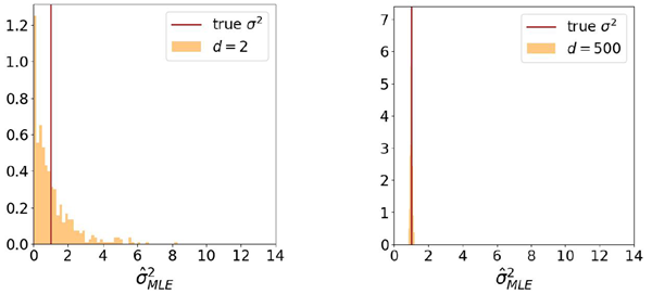
まず、\(p_X\) が \(\mathbb{R}^d\) の \(k\) 次元部分空間に支持された 2 成分ガウス分布である場合の解析的ブラインドデノイザーモデルを考察する。ここで、最適スコア関数 \(∇\log p_σ\) は閉形式で既知であり、ノイズ推定における不確実性によって生じる誤差を分離することができる。解析的ブラインドデノイザーは、ノイズサンプル \(y\) に対する µ(·|y) の最大尤度推定値 (MLE) で与えられる。 \] s^⋆(y) ≈ \hat{s}(y) := \hat{σ}^2∇\log p_σb(y),\quad \hat{σ} = \text{arg}\max µ(σ|y) \] Figure 1 shows the distribution of estimated noise values for a mixture of two Gaussians of dimensionality \(k\) in a \(d\)-dimensional ambient space. Estimates are broadly distributed when \(k ≈ d\), but concentrate when \(k^2 ≪ d\), illustrating a “blessing of di-mensionality”. Figure 2 shows samples generating via Algorithm 2 using our analytical denoiser. In these experiments, \(h = 0.3\) and the dynamics are deterministic (\(a_t = 0\)). Similar results are obtained when \(a_t > 0\). For more details, see Appendix G.1.
図1は、\(d\)次元のアンビエント空間における次元数\(k\)の2つのガウス分布の混合に対する推定ノイズ値の分布を示しています。推定値は\(k ≈ d\)の場合には広く分布しますが、\(k^2 ≪ d\)の場合には集中し、「次元性の恩恵」を示しています。図2は、解析的ノイズ除去器を用いてアルゴリズム2で生成されたサンプルを示しています。これらの実験では、\(h = 0.3\)であり、ダイナミクスは決定論的（\(a_t = 0\)）です。\(a_t > 0\)の場合も同様の結果が得られています。詳細については、付録G.1を参照してください。

Figure 1: Empirical density of maximum likelihood noise level estimates \(\hat{σ} = \text{arg}\max µ(σ|y)\) for a mixture of two Gaussian with intrinsic dimensionality \(k = 2\) in an ambient space of dimensionality \(d\). Estimates are broadly distributed when \(d = k\) (left), but highly concentrated when \(d ≫ k^2\) (right).
図1: 次元数\(d\)の環境空間における、固有次元数\(k = 2\)の2つのガウス分布の混合分布に対する最大尤度ノイズレベル推定値\(\hat{σ} = \text{arg}\max µ(σ|y)\)の経験的密度。推定値は\(d = k\)（左）の場合には広く分布しているが、\(d ≫ k^2\)（右）の場合には非常に集中している。

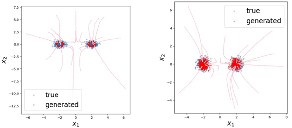
Figure 2: Example trajectories and samples for an analytical blind denoiser applied to a mixture of two Gaussians with \(k = 2\). For \(d = k = 2\) (left), sampling fails, due to errors in the MLE estimates of noise level. For \(d = 500 ≫ k^2\) (right), sampling is successful, illustrating the blessings of dimensionality.
図2: \(k = 2\)の2つのガウス分布の混合に解析的ブラインドノイズ除去を適用した場合の軌跡とサンプルの例。\(d = k = 2\)（左）の場合、ノイズレベルのMLE推定値の誤差によりサンプリングが失敗します。\(d = 500 ≫ k^2\)（右）の場合、サンプリングは成功し、次元化の恩恵を示しています。

Training denoisers on synthetic data 合成データによるノイズ除去装置のトレーニング

In Appendix G.2, we verify that training blind denoisers (via neural networks) can accurately sample from toy densities as well. Under an appropriate step-size choice of \(h = 0.5\) and \(a_s = \frac{1}{2}σ_t^2\) , we see that \(\hat{σ}_k \simeq σ_t\) as predicted by Proposition 3.2. Figure 3 demonstrates the benefits of having low intrinsic dimensionality for learning to sample Gaussian data, and similarly for Gaussian mixtures (see appendix for training details).
付録G.2では、ニューラルネットワークを用いたブラインドノイズ除去器の訓練によって、おもちゃの密度から正確にサンプリングできることを検証する。適切なステップサイズ \(h = 0.5\) および \(a_s = \frac{1}{2}σ_t^2\) を選択すると、命題3.2で予測される通り、 \(\hat{σ}_k \simeq σ_t\) となる。図3は、ガウス分布データのサンプリング学習において、固有次元が低いことの利点を示している。ガウス分布の混合分布についても同様である（訓練の詳細については付録を参照）。

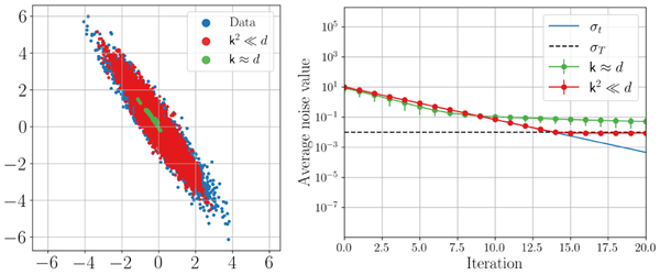
Figure 3: Sampling performance of BDDMs trained on Gaussian data with intrinsic dimension \(k = 2\) and two different input dimensions \(d ∈ \{2,100\}\). Generated samples (left) and evolution of the estimated noise level, corresponding to Proposition 3.2 (right).
図3: 固有次元 \(k = 2\) と2つの異なる入力次元 \(d ∈ \{2,100\}\) を持つガウスデータでトレーニングされたBDDMのサンプリング性能。生成されたサンプル（左）と命題3.2に対応する推定ノイズレベルの推移（右）。

4.2 Photographic images 写真画像

Do these results extend beyond the synthetic data to real-world models and signals? To investigate this question, we consider deep neural networks trained on natural images. We trained a non-blind and blind model to approximate the optimal denoisers in (5) and (9), respectively.
これらの結果は、合成データを超えて、現実世界のモデルや信号にも適用できるだろうか？この問いを検証するために、自然画像で学習したディープニューラルネットワークを考察する。(5)と(9)の最適ノイズ除去器を近似するために、それぞれ非ブラインドモデルとブラインドモデルを学習した。

Datasets.　Under the manifold hypothesis, natural images concentrate near a union of low-dimensional manifolds. This implies that natural images have low intrinsic dimensionality, making them a suitable testbed for our theoretical results. We use two popular image datasets, CelebA (Liu et al., 2015) with ≈ 200,000 images and a random subset of LSUN (bedroom class) data set with ≈ 300,000 images (Yu et al., 2015).
データセット：多様体仮説によれば、自然画像は低次元多様体の和集合付近に集中する。これは、自然画像の固有次元が低いことを意味し、我々の理論的結果の実験台として適している。我々は、2つの一般的な画像データセット、約20万枚の画像を含むCelebA（Liu et al., 2015）と、約30万枚の画像を含むLSUN（寝室クラス）データセットのランダムサブセット（Yu et al., 2015）を使用する。

These datasets are complex enough to capture real-world structure while remaining simple enough to train smaller-size networks without text conditioning. All images are downsampled to 80 × 80 resolution.
これらのデータセットは、現実世界の構造を捉えるのに十分な複雑さを持ちながら、テキスト条件付けなしで小規模なネットワークを学習できるほどシンプルです。すべての画像は80×80の解像度にダウンサンプリングされています。

Architecture and training.　UNet (Ronneberger et al., 2015) is the most popular denoising and score estimation architecture. For both blind and non-blind models, we use the simplest UNet architecture with 13 million parameters, and train all models from scratch. (We note that this architecture is quite small compared to others which use hundreds of millions of parameters). See Appendix G.3 for more details.
アーキテクチャとトレーニング UNet (Ronneberger et al., 2015) は、最も人気のあるノイズ除去およびスコア推定アーキテクチャです。ブラインドモデルと非ブラインドモデルの両方において、1,300万個のパラメータを持つ最もシンプルなUNetアーキテクチャを使用し、すべてのモデルをゼロからトレーニングしました。（このアーキテクチャは、数億個のパラメータを使用する他のアーキテクチャと比較すると非常に小さいことに注意してください。）詳細については、付録G.3を参照してください。

Can the noise level be accurately estimated from a single noisy image by a trained neural network denoiser? If natural images are truly low dimensional, then we expect \(µ(σ|x_σ) ≃ δ_σ\). Additionally, the inductive biases of the neural network should allow for leveraging the concentration to get a precise estimate of true variance. If both of these conditions are satisfied, then the performance gap between blind and non-blind denoisers will be small. Figure 4 compares denoising error of the two models on two datasets in terms of their peak signal-to-noise ratio (PSNR) averaged across the data, written \(PSNR(x,\hat{x}) := −10\log_{10}||x−\hat{x}||^2\), where \(\hat{x}\) is the output of a blind or non-blind denoiser. The two plots clearly display that both blind and non-blind denoisers have the same “one-shot” denoising ability, as their denoising errors are virtually identical.
訓練されたニューラルネットワークのノイズ除去装置によって、単一のノイズ画像からノイズレベルを正確に推定できるでしょうか? 自然画像が本当に低次元であれば、\(µ(σ|x_σ) ≃ δ_σ\) が期待できます。さらに、ニューラルネットワークの誘導バイアスにより、集中度を利用して真の分散を正確に推定できるようになります。これらの条件が両方とも満たされている場合、ブラインドノイズ除去装置と非ブラインドノイズ除去装置のパフォーマンスの差は小さくなります。図 4 は、2 つのデータセットに対する 2 つのモデルのノイズ除去誤差を、データ全体で平均したピーク信号対ノイズ比 (PSNR) で比較しています。PSNR は \(PSNR(x,\hat{x}) := −10\log_{10}||x−\hat{x}||^2\) と表記され、\(\hat{x}\) はブラインドまたは非ブラインドノイズ除去装置の出力です。 2 つのグラフは、ブラインドデノイザーと非ブラインドデノイザーの両方のノイズ除去エラーが実質的に同じであるため、同じ「ワンショット」ノイズ除去機能を備えていることを明確に示しています。

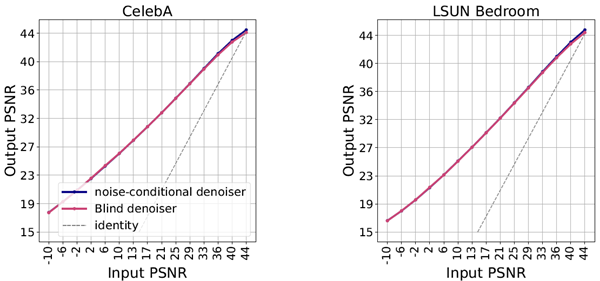
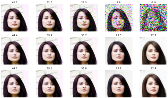
Figure 4: Top panel. Comparison of denoising performance of blind and non-blind denoisers. Performance is evaluated on the test sets of CelebA and Bedroom class of LSUN datasets, and is reported in terms of PSNR. For consistency, the noise level on the horizontal axis is also expressed as PSNR(\(x,x_σ\)). Bottom panel. An example test image with corresponding PSNR values. Top: Noisy images. Middle: Denoised image by a non-blind denoiser. Bottom: Denoised image by a blind denoiser.
図4：上段。ブラインドデノイザーと非ブラインドデノイザーのノイズ除去性能の比較。性能は、CelebAクラスとBedroomクラスのLSUNデータセットのテストセットで評価され、PSNRで報告されています。一貫性を保つため、横軸のノイズレベルはPSNR(\(x,x_σ\))とも表記されています。下段。対応するPSNR値を示すテスト画像の例。上段：ノイズを含む画像。中段：非ブラインドデノイザーによるノイズ除去画像。下段：ブラインドデノイザーによるノイズ除去画像。

Now we sample from \(\hat{p}_T ≈ p_X\) learned by the models via Algorithm 2. Hyperparam-eters are set to \(σ_{max} = 4,σ_{min} = 0.05,h = 0.2,a_t = 0.2\hat{σ}_t\), which leads to a total number of steps \(N ≈ 100\). We compare to the non-blind denoisers through the variance exploding (VE) DDPM algorithm (Song et al., 2021a), with a \(\log σ\) schedule with \(N = 100\).
ここで、アルゴリズム2を用いてモデルが学習した\(\hat{p}_T ≈ p_X\)からサンプリングを行います。ハイパーパラメータは\(σ_{max} = 4,σ_{min} = 0.05,h = 0.2,a_t = 0.2\hat{σ}_t\)に設定され、合計ステップ数は\(N ≈ 100\)となります。分散爆発(VE)DDPMアルゴリズム(Song et al., 2021a)を用いて、\(\log σ\)スケジュールで\(N = 100\)、非ブラインドデノイザーと比較します。

Figures 5 shows samples from both algorithms (see Figure 7 for additional examples and Figure 8 for LSUN samples). Surprisingly, samples generated by BDDMs appear to have higher visual quality than samples generated by the non-blind DDMs. This suggests that the distribution of BDDM samples is closer to the true image density than that of DDPM samples.
図5は、両方のアルゴリズムによるサンプルを示しています（追加例は図7、LSUNサンプルは図8を参照）。驚くべきことに、BDDMによって生成されたサンプルは、非ブラインドDDMによって生成されたサンプルよりも視覚品質が高いようです。これは、BDDMサンプルの分布がDDPMサンプルよりも真の画像密度に近いことを示唆しています。

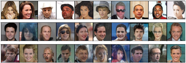
Figure 5: Comparison of samples from BDDM and VE-DDPM. Top row: Randomly selected subset of training images from the celebA dataset. Second row: Samples generated by BDDM with \(N ≈ 100\). Third row: Samples generated by a non-blind DDM (VE-DDPM) with \(N = 100\). Samples in each column are initialized with the same random seed, and use matched injected noise. Seeds are random and not curated for quality.
図5: BDDMとVE-DDPMのサンプルの比較。上段: celebAデータセットからランダムに選択されたトレーニング画像のサブセット。2段目: BDDM（N ≈ 100）で生成されたサンプル。3段目: 非ブラインドDDM（VE-DDPM）（N = 100）で生成されたサンプル。各列のサンプルは同じランダムシードで初期化され、一致するノイズが注入されています。シードはランダムであり、品質を考慮してキュレーションされていません。

We hypothesize that using non-blind models in a backward process with an explicit schedule incurs a mismatch error: the “true” noise level on the image diverges from the noise level dictated by the schedule of the algorithm. Figure 6 illustrates the nature of the mismatch error in one-shot denoising in a non-blind model. Each plot shows the mean-squared error (MSE) between denoised and clean images, as a function of the second argument. MSE is lowest when the second argument is equal to the “true” noise level, \(σ = σ^⋆\). If the argument σ is too small, the denoised image is noisier than that of the cor-rect denoiser; too large, and the image is more blurred than that of the correct denoiser.
我々は、明示的なスケジュールによる後方処理で非ブラインドモデルを使用すると、ミスマッチエラーが発生するという仮説を立てています。つまり、画像の「真の」ノイズレベルが、アルゴリズムのスケジュールによって指示されたノイズレベルから逸脱するということです。図 6 は、非ブラインドモデルでのワンショットノイズ除去におけるミスマッチエラーの性質を示しています。各プロットは、ノイズ除去された画像とクリーンな画像の平均二乗誤差 (MSE) を、2 番目の引数の関数として示しています。MSE は、2 番目の引数が「真の」ノイズレベルに等しい場合 (σ = σ^⋆)、最も低くなります。引数 σ が小さすぎると、ノイズ除去された画像は正しいノイズ除去の画像よりもノイズが多くなります。引数 σ が大きすぎると、画像は正しいノイズ除去の画像よりもぼやけた画像になります。

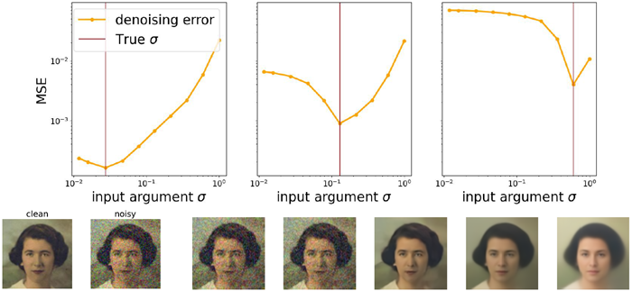
Figure 6: Sensitivity of non-blind denoising performance to mismatches in true noise level and argument to the denoiser. Top row: Denoising error (averaged over 512 samples) as a function of argument \(σ\) for three different true noise levels (from left to right, \(σ^⋆ ∈ [0.025,0.15,0.6])\). Bottom row: Example clean image x0, noisy image \(x_{σ^⋆} = x_0 + σ^⋆z\), for \(σ^⋆ = 0.1\), and five images resulting from a non-blind denoiser \(\tilde{x} = \tilde{f}_θ(x_{σ^⋆} ,σ)\) with \(σ ∈ [0.01,0.03,0.10,0.32,1.0]\) (from left to right).
図6: 真のノイズレベルとノイズ除去器への引数の不一致に対する非ブラインドノイズ除去性能の感度。上段: 3つの異なる真のノイズレベル（左から右へ、\(σ^⋆ ∈ [0.025,0.15,0.6])\)における引数\(σ\)の関数としてのノイズ除去誤差（512サンプルの平均）下の行: クリーンな画像 x0 の例、ノイズのある画像 \(x_{σ^⋆} = x_0 + σ^⋆z\) (\(σ^⋆ = 0.1\))、および非ブラインドノイズ除去 \(\tilde{x} = \tilde{f}_θ(x_{σ^⋆} ,σ)\) (\(σ ∈ [0.01,0.03,0.10,0.32,1.0]\) の結果の 5 つの画像 (左から右へ)。

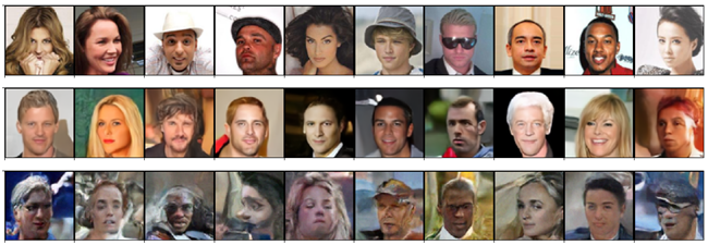
Figure 7: Higher number of steps \(N ≈ 17000\) improves quality of samples for all models shown in Fig. 5. The samples from BDDM are still of significantly higher quality than samples from DDPM. Samples in each column are initialized with the same random seed with matched injected noise.
図7：ステップ数を増やす（N ≈ 17000）と、図5に示すすべてのモデルのサンプル品質が向上します。BDDMのサンプルは、DDPMのサンプルよりも依然として大幅に高い品質です。各列のサンプルは、同じ乱数シードと、それに対応するノイズ注入で初期化されています。

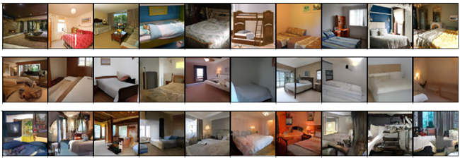
Figure 8: Top row: example training images from the LSUN dataste. Second row: samples generated by BDDM with average number of steps \(N ≈ 1300\). Third row: Samples generated by DDPM (VE) algorithm, with total number of steps \(N = 1300\). Samples in each column are initialized with the same random seed with matched injected noise.
図8：上段：LSUNデータセットのトレーニング画像例。2段目：平均ステップ数（N ≈ 1300）でBDDMアルゴリズムによって生成されたサンプル。3段目：総ステップ数（N = 1300）でDDPM（VE）アルゴリズムによって生成されたサンプル。各列のサンプルは、同じ乱数シードと、対応するノイズが注入された状態で初期化されている。

To quantify the mismatch in the DDPM backward sampling process, we train a separate small neural network to estimate the noise level of an image—a much simpler task than denoising. Figure 12 in the appendix shows that this network produces highly accurate estimates of noise level, confirming the concentration of the likelihood. We can use this network to estimate the true noise level of the intermediate samples generated by DDPM, and compare them to the \(σ\) imposed by the schedule.
DDPMの逆方向サンプリング処理におけるミスマッチを定量化するために、画像のノイズレベルを推定する別の小規模ニューラルネットワークをトレーニングします。これはノイズ除去よりもはるかに単純なタスクです。付録の図12は、このネットワークが非常に正確なノイズレベル推定値を生成することを示しており、尤度の集中を裏付けています。このネットワークを使用して、DDPMによって生成される中間サンプルの真のノイズレベルを推定し、スケジュールによって課される\(σ\)と比較することができます。

Figure 9 shows that scheduled noise levels systemically fall behind the true noise value of the image. This suggests that the low quality of the samples in Figure 5 results from a mismatch error in which \(σ_t \gt σ^⋆\) along the trajectory. Per the left-most plot in Figure 9, this same noise-estimator model shows that, BDDMs precisely track the implicit schedule of the backward process. Moreover, given our theoretical results, we can conclude that the only reason DDPM fails to generate images in the constant stepsize regime is precisely due to this mismatch which is not observed in BDDMs (see third row of Figure 5).
図9は、スケジュールされたノイズレベルが画像の真のノイズ値よりも系統的に遅れていることを示しています。これは、図5のサンプルの低品質は、軌跡に沿って\(σ_t \gt σ^⋆\) となるミスマッチ誤差に起因していることを示唆しています。図9の左端のプロットによれば、この同じノイズ推定モデルは、BDDMが後方プロセスの暗黙的なスケジュールを正確に追跡していることを示しています。さらに、理論的な結果を考慮すると、DDPMが一定ステップサイズ領域で画像を生成できない唯一の理由は、まさにこのミスマッチによるものであり、BDDMでは観察されないと結論付けることができます（図5の3行目を参照）。

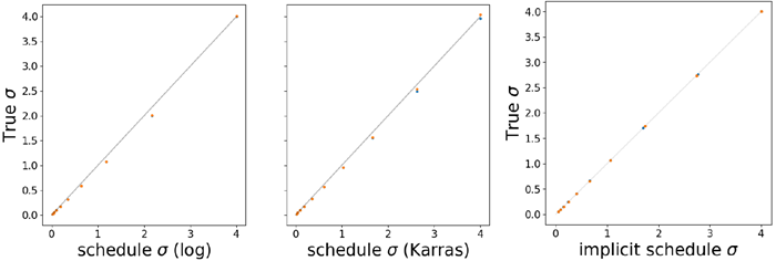
Figure 9: Empirical comparison of scheduled noise level \(σ_t\) and estimated noise level \(σ^⋆\) along trajectories of 50 steps for 2 samples. Every 5 steps is shown. The DDPM backward process outpaces a log schedule (left), or the schedule proposed by Karras et al. (2022) (middle), leading to an excess error manifested in the lower quality of samples. In contrast, BDDM accurately tracks the implicit schedule \(σ_t\) via \(\hat{σ}_k = ||x_k − \hat{f}_θ(x_k)||/\sqrt{d}\). Adaptivity of step size to underlying sample is demonstrated. (right).
図9: 2つのサンプルについて50ステップの軌跡に沿ったスケジュールされたノイズレベル \(σ_t\) と推定されたノイズレベル\(σ^⋆\)の実験的比較。5ステップごとに表示されています。DDPMの逆方向プロセスは、対数スケジュール（左）またはKarras et al. (2022)が提案したスケジュール（中央）よりも速く、サンプルの品質が低下するという形で過剰な誤差が生じます。対照的に、BDDMは\(\hat{σ}_k = ||x_k − \hat{f}_θ(x_k)||/\sqrt{d}\)を介して暗黙のスケジュール\(σ_t\)を正確に追跡します。ステップサイズが基礎サンプルに適応していることが示されています。（右）。

5 Conclusion 結論

This work presents a comprehensive mathematical analysis and justification of blind denoising diffusion models, closing a gap in the literature. We identify low intrinsic dimensionality of the underlying data distribution, which allows the denoiser to (im-plicitly) estimate noise level from an image, as a critical component underlying the success of these models both theoretically and empirically. A key consequence is that, unlike e.g., DDPM, we prove that a constant stepsize schedule sufices to sample data distributions via BDDMs. Moreover, we have shown that BDDM models can offer improved sample quality by avoiding errors due to mismatch in noise schedules. The use of BDDMs merit further investigation at larger scales, as well as in application to other downstream tasks such as fine-tuning and inverse problems.
本研究では、ブラインドノイズ除去拡散モデルの包括的な数学的解析と正当性を示し、文献の空白を埋める。我々は、基礎となるデータ分布の低い固有次元（これにより、ノイズ除去装置が画像からノイズレベルを（暗黙的に）推定することを可能にする）が、これらのモデルの理論的および経験的成功の根底にある重要な要素であると特定した。重要な結論として、例えばDDPMとは異なり、BDDMを介したデータ分布のサンプリングには一定のステップサイズスケジュールで十分であることを証明した。さらに、BDDMモデルはノイズスケジュールの不一致によるエラーを回避することで、サンプル品質を向上させることができることを示した。BDDMの使用は、より大規模な研究、および微調整や逆問題などの他の下流タスクへの応用に価値がある。

Acknowledgements 謝辞

ZK acknowledges the computing facilities of the Flatiron Institute. AAP acknowledges the Yale Institute for the Foundations of Data Science for financial support.
ZKはフラットアイアン研究所のコンピューティング設備に感謝の意を表します。AAPはイェール大学データサイエンス基礎研究所の財政支援に感謝の意を表します。

References 参考文献

Arjovsky, M., Chintala, S., and Bottou, L. (2017). Wasserstein generative adversarial networks. Proceedings of the 34th International Conference on Machine Learning, 70:214–223.
『Wasserstein生成的敵対的ネットワーク』

Benton, J., De Bortoli, V., Doucet, A., and Deligiannidis, G. (2024). Nearly d-linear convergence bounds for diffusion models via stochastic localization. In The Twelfth International Conference on Learning Representations.
『確率的局所化による拡散モデルの近似d線型収束限界』

Brown, B. C., Caterini, A. L., Ross, B. L., Cresswell, J. C., and Loaiza-Ganem, G. (2023). Verifying the union of manifolds hypothesis for image data. In The Eleventh International Conference on Learning Representations.
『画像データにおける多様体和集合仮説の検証』

Chandler, D. M. and Field, D. J. (2007). Estimates of the information content and dimensionality of natural scenes from proximity distributions. Journal of the Optical Society of America A, 24(4):922–941.
『近接分布を用いた自然風景の情報量と次元数の推定』

Chen, F., Chewi, S., Daskalakis, C., and Rakhlin, A. (2026). High-accuracy sampling for diffusion models and log-concave distributions. arXiv preprint 2602.01338.
『拡散モデルと対数凹分布のための高精度サンプリング』

Chen, S., Chewi, S., Li, J., Li, Y., Salim, A., and Zhang, A. (2023). Sampling is as easy as learning the score: Theory for diffusion models with minimal data assumptions. In The Eleventh International Conference on Learning Representations.
『サンプリングはスコアの学習と同じくらい簡単：最小限のデータ仮定を用いた拡散モデルの理論』

Conforti, G., Durmus, A., and Silveri, M. G. (2025). KL convergence guarantees for score diffusion models under minimal data assumptions. SIAM Journal on Mathematics of Data Science, 7(1):86–109.
『最小データ仮定下におけるスコア拡散モデルのKL収束保証』

Efron, B. (2011). Tweedie’s formula and selection bias. Journal of the American Statistical Association, 106(496):1602–1614.
『トゥイーディーの公式と選択バイアス』

Föllmer, H. (1985). An entropy approach to the time reversal of diffusion processes. In Stochastic differential systems (Marseille-Luminy, 1984), volume 69 of Lect. Notes Control Inf. Sci., pages 156–163. Springer, Berlin.
『拡散過程の時間反転に対するエントロピーアプローチ』

Gatmiry, K., Chen, S., and Salim, A. (2026). High-accuracy and dimension-free sampling with diffusions. arXiv preprint arXiv:2601.10708.
『拡散法を用いた高精度かつ次元フリーなサンプリング』

Grathwohl, W., Chen, R. T. Q., Bettencourt, J., and Duvenaud, D. (2019). FFJORD: free-form continuous dynamics for scalable reversible generative models. In International Conference on Learning Representations.
『スケーラブルで可逆な生成モデルのための自由形式連続ダイナミクス』

H´enaff, O. J., Ball´e, J., Rabinowitz, N. C., and Simoncelli, E. P. (2014). The local low-dimensionality of natural images. CoRR, abs/1412.6626.
『自然画像の局所的低次元性』

Ho, J., Jain, A., and Abbeel, P. (2020). Denoising diffusion probabilistic models. Advances in neural information processing systems, 33:6840–6851.
『拡散確率モデルのノイズ除去』

Huang, Z., Wei, Y., and Chen, Y. (2024). Denoising diffusion probabilistic models are optimally adaptive to unknown low dimensionality. arXiv preprint arXiv:2410.18784.
『ノイズ除去拡散確率モデルは未知の低次元に対して最適適応性を示す』

Kadkhodaie, Z., Guth, F., Simoncelli, E. P., and Mallat, S. (2024). Generalization in diffusion models arises from geometry-adaptive harmonic representations. In The Twelfth International Conference on Learning Representations.
『拡散モデルにおける一般化は、幾何学適応型調和表現から生じる』

Kadkhodaie, Z. and Simoncelli, E. (2021). Stochastic solutions for linear inverse problems using the prior implicit in a denoiser. Advances in Neural Information Processing Systems, 34:13242–13254.
『ノイズ除去装置における事前分布を用いた線形逆問題の確率的解法』

Kadkhodaie, Z. and Simoncelli, E. P. (2020). Solving linear inverse problems using the prior implicit in a denoiser. arXiv preprint arXiv:2007.13640.
『ノイズ除去器における事前分布を用いた線形逆問題の解法』

Karras, T., Aittala, M., Aila, T., and Laine, S. (2022). Elucidating the design space of diffusion-based generative models. Advances in neural information processing systems, 35:26565–26577.
『拡散に基づく生成モデルの設計空間の解明』

Kingma, D. P. and Welling, M. (2013). Auto-encoding variational bayes. arXiv preprint arXiv:1312.6114.
『オートエンコーディング変分ベイズ』

Lee, H., Lu, J., and Tan, Y. (2023). Convergence of score-based generative modeling for general data distributions. In International Conference on Algorithmic Learning Theory, pages 946–985. PMLR.
『一般データ分布に対するスコアベース生成モデリングの収束』

Li, G. and Yan, Y. (2024). Adapting to unknown low-dimensional structures in score-based diffusion models. Advances in Neural Information Processing Systems, 37:126297–126331.
『スコアベース拡散モデルにおける未知の低次元構造への適応』

Li, T. and He, K. (2025). Back to basics: let denoising generative models denoise. arXiv preprint arXiv:2511.13720.
『基本に立ち返る：生成モデルのノイズ除去』

Liang, J., Huang, Z., and Chen, Y. (2025). Low-dimensional adaptation of diffusion models: Convergence in total variation (extended abstract). In Proceedings of Thirty Eighth Conference on Learning Theory, volume 291 of Proceedings of Machine Learning Research. PMLR.
『拡散モデルの低次元適応：トータルバリエーションにおける収束』

Liu, Z., Luo, P., Wang, X., and Tang, X. (2015). Deep learning face attributes in the wild. In Proceedings of International Conference on Computer Vision (ICCV).
『ディープラーニングによる顔属性の実環境への適用』

Miyasawa, K. (1961). An empirical Bayes estimator of the mean of a normal population. Bull. Inst. Internat. Statist., 38:181–188.
『正規分布の平均値の経験的ベイズ推定量』

Olshausen, B. A. and Field, D. J. (1996). Natural image statistics and eficient coding. Network: computation in neural systems, 7(2):333.
『自然画像統計と効率的な符号化. ネットワーク』

Pooladian, A.-A. and Niles-Weed, J. (2025). Plug-in estimation of Schro¨dinger bridges. SIAM Journal on Mathematics of Data Science, 7(3):1315–1336.
『シュレーディンガーブリッジのプラグイン推定』

Pope, P., Zhu, C., Abdelkader, A., Goldblum, M., and Goldstein, T. (2021). The intrinsic dimension of images and its impact on learning. In International Conference on Learning Representations.
『イメージの内在的次元と学習への影響』

Potaptchik, P., Azangulov, I., and Deligiannidis, G. (2024). Linear convergence of diffusion models under the manifold hypothesis. arXiv preprint arXiv:2410.09046.
『多様体仮説下における拡散モデルの線形収束』

Raphan, M. and Simoncelli, E. P. (2011). Least squares estimation without priors or supervision. Neural Computation, 23(2):374–420.
『事前分布や教師なしの最小二乗推定』

Ronneberger, O., Fischer, P., and Brox, T. (2015). U-net: convolutional networks for biomedical image segmentation. In Int’l Conf Medical Image Computing and Computer-assisted Intervention, pages 234–241. Springer.
『U-net: バイオメディカル画像セグメンテーションのための畳み込みネットワーク』

Roweis, S. T. and Saul, L. K. (2000). Nonlinear dimensionality reduction by locally linear embedding. Science, 290(5500):2323–2326.
『局所線形埋め込みによる非線形次元削減』

Sohl-Dickstein, J., Weiss, E., Maheswaranathan, N., and Ganguli, S. (2015). Deep unsupervised learning using nonequilibrium thermodynamics. In International Conference on Machine Learning, pages 2256–2265. PMLR.
『非平衡熱力学を用いた教師なし深層学習』

Song, J., Meng, C., and Ermon, S. (2021a). Denoising diffusion implicit models. In International Conference on Learning Representations.
『拡散暗黙モデルのノイズ除去』

Song, Y., Sohl-Dickstein, J., Kingma, D. P., Kumar, A., Ermon, S., and Poole, B. (2021b). Score-based generative modeling through stochastic differential equations. In International Conference on Learning Representations.
『確率微分方程式によるスコアベースの生成モデリング』

Sun, Q., Jiang, Z., Zhao, H., and He, K. (2025). Is noise conditioning necessary for denoising generative models? In Forty-second International Conference on Machine Learning.
『生成モデルのノイズ除去にはノイズ調整は必要か？』

Tang, J. and Yan, Y. (2025). Adaptivity and convergence of probability flow ODEs in diffusion generative models. arXiv preprint arXiv:2501.18863.
『拡散生成モデルにおける確率フロー常微分方程式の適応性と収束性』

Wang, R. and Du, Y. (2025). Equilibrium matching: generative modeling with implicit energy-based models. arXiv preprint arXiv:2510.02300.
『平衡マッチング：暗黙的エネルギーベースモデルを用いた生成モデリング』

Yu, F., Seff, A., Zhang, Y., Song, S., Funkhouser, T., and Xiao, J. (2015). LSUN: construction of a large-scale image dataset using deep learning with humans in the loop. arXiv preprint arXiv:1506.03365.
『人間を巻き込んだディープラーニングによる大規模画像データセットの構築』

Zhang, K., Zuo, W., Chen, Y., Meng, D., and Zhang, L. (2017). Beyond a Gaussian denoiser: residual learning of deep CNN for image denoising. IEEE Transactions on Image Processing, 26(7):3142–3155.
『ガウス分布ノイズ除去を超えて：画像ノイズ除去のための深層CNNの残差学習』

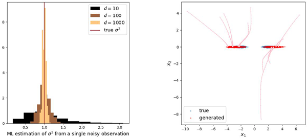
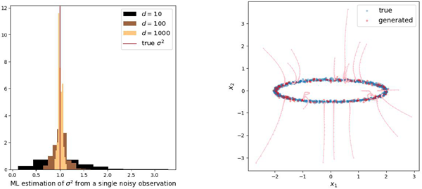
Figure 10: Top: Mixture of two Gaussians with covariances of rank \(k = 1\). On the left, the effect of increasing ambient dimensionality, \(d\) is shown. On the right, sampling is shown for \(d = 1000\). Bottom: Ellipse constructed as a mixture of Gaussians. Sampling is shown for \(d = 100\).
図10：上：共分散がランク \(k = 1\) の2つのガウス分布の混合。左側は、周囲次元 \(d\) の増加による効果を示す。右側は、\(d = 1000\) のサンプリング結果を示す。下：ガウス分布の混合として構築された楕円。\(d = 100\) のサンプリング結果を示す。

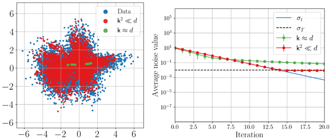
Figure 11: Sampling performance of BDDMs trained on a mixture of Gaussian datset a with intrinsic dimension \(k = 2\) and two different input dimensions \(d ∈ {2, 200}\). Generated samples (left) and evolution of the estimated noise level, corresponding to Proposition 3.2 (right).
図11: 固有次元 \(k = 2\) を持つガウスデータセット a と2つの異なる入力次元 \(d ∈ {2, 200}\) の混合データで学習したBDDMのサンプリング性能。生成されたサンプル（左）と、命題3.2に対応する推定ノイズレベルの推移（右）。

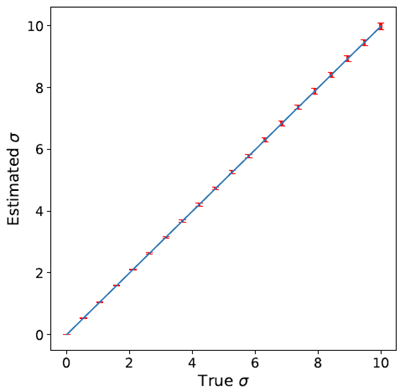
Figure 12: A smaller neural network trained to estimate \(σ\) from noisy image is very accurate. Error bars show two standard deviation. It is also worth noting that the model performs well beyond training range \(σ ∈ (0, 3]\).
図12: ノイズの多い画像から\(σ\)を推定するように訓練された小規模なニューラルネットワークは非常に正確です。エラーバーは2標準偏差を示しています。また、このモデルが訓練範囲\(σ ∈ (0, 3]\)を超えて良好なパフォーマンスを示していることも注目に値します。

A Proofs for Sections 3.1 and 3.2

A.1 Proof of Proposition 3.1

The population counterpart to (6) is
\[ f^⋆ = \text{arg}\min\limits_{f:\mathbb{R}^d→\mathbb{R}^d} \underset{\substack{σ∼Θ\\z∼γ}}{\mathbb{E}_{x∼p_X}}||x − f(x + σz)||^2\] Let \(y := x+σz\). The optimal function \(f\) of \(y\) to predict \(x\) is the conditional expectation \(\mathbb{E}[x|y]\), due to orthogonality:
\[ \mathbb{E}||x − f(y)||^2 = \mathbb{E}||x − \mathbb{E}[x|y]||^2 + \mathbb{E}||\mathbb{E}[x|y] − f(y)||^2 \tag{16} \] On the other hand, by Bayes, we can express
\[ \mathbb{E}[x|y] = \int \mathbb{E}[x|σ,y]dµ(σ|y) \] Applying Tweedie’s identity (5),
\[ \mathbb{E}[x|y] = \int (y + σ^2∇\log p_σ(y)dµ(σ|y) \] We remark that by (16), for any estimator \(\hat{f}\), the excess risk is
\[ \begin{align} \mathcal{E}(f) &:= \mathbb{E}||x −\hat{f}(y)||^2 − \mathbb{E}||x − f^⋆(y)||^2 \\ \\ &= \mathbb{E}||\hat{f}(y) − f^⋆(y)||^2= \int ||\hat{f} − f^⋆||_{L^2(p_σ)}^2 dΘ(σ) \end{align} \tag{17} \]

A.2 Proof of Proposition 3.2

Let \(ρ_t := \text{Law}(X_t)\) and \(\tilde{ρ}_t := p_{σ_t}:= p_X ∗ γ_{σ_t^2}\). We first compute directly \(∂_t\tilde{ρ}_t\) from this definition using the fact that the Gaussian density is the solution to the heat equation:
\[ \begin{align} ∂_t\tilde{ρ}_t(y) &= ∂_t \int γ_{σ_t^2}(y)p_X(y − x)dx \\ \\ &= \int (∂_tγ_{σ_t^2}(y))p_X(y − x)dx \\ \\ &= \int(∂_tσ_t^2) (∂_sγ_s|_{s=σ_t^2}(y)) p_X(y − x) dx \\ \\ &=\frac{1}{2}(∂_tσ_t^2 ) \int Δγ_{σ_t^2}(y) p_X(y − x) dx \\ \\ &= \frac{1}{2}(∂_tσ_t^2)Δ_y \int γ_{σ_t^2}(y) pX(y − x) dx \\ \\ &= \frac{1}{2}(∂_tσ_t^2)Δ\tilde{ρ}_t(y) \tag{18} \end{align} \] On the other hand, under the ideal dynamics (11), the Fokker–Planck equation reads
\[ \begin{align} ∂_tρ_t &= −∇ · (ρ_tσ_t^2 ∇\log p_{σ_t}) + a_t ∆_{ρ_t} \\ \\ &= −∇ · (ρ_tσ_t^2 ∇\log\tilde{ρ}_t) + a_t ∆_{ρ_t} \end{align} \tag{19} \] Since \(∆\tilde{ρ}_t = ∇·(\tilde{ρ}_t∇\log\tilde{ρ}_t)\), (18) shows that \((\tilde{ρ}_t)_{t∈[0,T]}\) solves the equation (19), provided that
\[ \frac{1}{2}(∂_tσ_t^2) = −σ_t^t + a_t \tag{20} \] By uniqueness of solutions to the Fokker–Planck equation, we see that with this choice of \((σ_t)_{t∈[0,T]}\) and for \(ρ_0 = \tilde{ρ}_0\), we have \(ρ_t = \tilde{ρ}_t\) for all \(t ∈ [0,T]\). Solving the ODE (20) yields the claim.

A.3 Proof of Lemma 3.3

Recall that \(\frac{1}{2}∂_t(σ_t^2) = −σ_t^2 + a_t\), so we want to show \(a_t ≤ σ_t^2\) for all \(t ≥ 0\). Note that if \(a_t ≤ a_0 ≤ σ_0~2\) for all \(t ≥ 0\), then
\[ σ_t^2 = σ_0^2 e^{−2t} + 2 \int_0^t a_s e^{−2(t−s)} ds ≥ σ_0^2 e^{−2t} + a_t(1 − e^{−2t}) \] This is lower bounded by \(a_t\) provided \(a_t ≤ σ_0^2\).

A.4 Proof of Lemma 3.4

The first term in Proposition 3.2 is obviously decaying to zero, so we must show that \(2\int_0^t a_s e^{−2(t−s)} ds → 0\). Since \(a_t → 0\), for any \(ε > 0\) there exists \(t_0\) such that \(a_t ≤ ε\) for all \(t ≥ t_0\). Then, for \(t ≥ t_0\,
\[ \begin{align} \int_0^t 2a_se^{−2(t−s)} ds &≤ \int_0^{t_0} (···) + \int_{t_0}^t (···)\\ \\ &≤ a_0 (e^{−2(t−t_0)} − e^{−2t}) + ε(1 − e^{−2(t−t_0)})\\ \\ &≤ a_0 (e^{−2(t−t_0)} − e^{−2t}) + ε \end{align} \] We can choose t suficiently large to make the first term at most ε as well.

B Proofs for Sections 3.3 and 3.4

B.1 Bound on the cross-covariance

Proposition B.1.　Under (A1) and (A2), for \(X_t ∼ p_{σ_t}\), with high probability,
\[ ||W_ω(X_t)|| ≲ (σ_t^2 + ω^2)(R +\sqrt{k})k \] Moreover, \[ \mathbb{E} \int \left| \int_σ^{σ_t} ||W_ω(X_t)||ω^{−3} dω\right|^2 dµ(σ|X_t) ≲_{\log} (R^2 + k)k^2 \mathbb{E} \int(|1 − σ_t^2/σ^2|^2 + |\log(σ_t/σ)|^2 dµ(σ|X_t) \] Proof. Recall that
\[ ∂_ω(ω^2∇\log p_ω(y)) = ω^{−3}W_ω(y):= ω^{−3}Cov_{q_ω}(X,||Y − X||^2|Y = y) \tag{21} \] By Lemma F.4, it holds that
\[ ||W_ω(X_t)|| ≲ (R^2 tr^2 C_ω(X_t) + tr C_ω(X_t)Q_ω(X,X_t)^{1/2} \tag{22} \] By applying Proposition F.2 (specifically Corollary F.3), on an event \(\mathcal{G}\) of probability \(1 − δ\), we have that
\[ ||W_ω(X_t)|| ≲ ((R^2 (σ_t^2 + ω^2)^2 k_δ^2 + (σ_t^2 + ω^2)^2 k_δ^3)^{1/2} ≲ (σ_t^2 + ω^2)k_δ (R +\sqrt{k_δ}) \] whence (again, on \(\mathcal{G}\))
\[ \begin{align} Z σ Z σ Z σ 2 2 δ t t t ∥Wω(Xt)∥ω−3 dω ≲ k2 (R2 + kδ) σ2ω−3 dω + ω−1 dω t σ σ σ ≲ k2 (R2 + kδ) |1 − σ2/σ2|2 + |log(σt/σ)|2 . t δ On the bad event, (22) implies ∥Wω(Xt)∥ ≲ R3 + R2 ∥Xt − X∥. Hence, hZ Z σ i 2 t E ∥Wω(Xt)∥ω−3 dω dµ(σ|Xt)1Gc σ ≲ Eh(R6 + R4 ∥Xt − X∥2)Z Z σt ω−3 dω2 dµ(σ|Xt)1Gci ≲ EhR6 + R4 ∥Xt − X∥2 1Gci σ σ 4 T ≲ sEhR12 + R8 ∥Xt − X∥4 iP(Gc) T σ 8 ≲ R6 + σ4R8d2 δ1/2 . T 0 σ 8 This term is negligible by choosing δ suficiently small. 24 B.2 Proof of Lemma 3.7 The change-of-variables formula is straightforward as |dλ| = 2λ−3/2. For the next part, dσ 1 we write ℓ(λ|y) = −logν(λ|y) = −d − α logλ − logEX∼pX exp −λ∥X − y∥ + c, 2 2 where c > 0 is an absolute constant. We compute via chain rule ℓ′(λ|y) = −d − α + 2 Eqλ[∥X − Y ∥2|Y = y], 1 2λ λ 1 where qλ(x|y) ∝ exp −2 ∥x − y∥2)pX(x), with ∂λqλ(x|y) = −2∥x − y∥2qλ. The second derivative is similar: ℓ′′(λ|y) = d2λ α − 4 Varqλ[∥X − Y ∥2|Y = y]. − 2 1 B.3 Proof of Proposition 3.8 Claim 1. ν(·|Xt) concentrates around λt with high probability. Proof of Claim 1. By Proposition F.2, with probability at least 1 − δ, ℓ′(λ|Xt) = −d + α + Eq [∥X − Y ∥2|Y = Xt] λ λ = −d ± O(kδ) + d ± O(pdlog(1/δ) + kδ)) . t λ λ Define the error term E = pdlog(1/δ) + kδ . Note that for λ > λ , ℓ′(λ|Xt) ≥ λt h1 − λt − O(E)i ≳ (d(λt− λt)/λ2 , t d t λ d d/λ , λtE/d ≪ λ − λt ≤ λt , λ − λt ≥ λt , where we require that E/d ≪ 1, i.e., d ≫log k. Therefore, for a ≫ λtE/d, we can integrate to find that Z ∞ Z 2λ t dν(λ|Xt) ≤ ν(λt|Xt)exp(−Ω(d(λ − λt)2/λ2))dλ λt+a λt+a t Z λmax + ν(λt|Xt)exp(−Ω(d))dλ h 2λt i λ t ≲ ad1/2 exp(−Ω(da2/λ2)) + λmax exp(−Ω(d)) ν(λt|Xt). On the other hand, for |λ − λt| ≪ λtE/d, one has |ℓ′(λ|Xt)| ≲ E/λt. Hence, t Z ν(λt|Xt) ≲ d ν(λt|Xt)dλ λ E t Z|λ−λt|≤cλtE/d d λ E ≲ ν(λ|Xt)exp(O(E(λ − λt)/λt))dλ t |λ−λt|≤cλtE/d ≲ E2 exp(O(E2/d)), d 25 and thus Z ∞ 1/2 t λ d t max λ d a E 2 dν(λ|Xt) ≲ exp(O(E2/d) − Ω(da2/λ2)) + exp(O(E2/d) − Ω(d)). λt+a If d ≫ k and we choose a ≫ λtE/d up to logarithmic factors, this shows that with very high probability under ν(· | Xt), h i λ ≤ λt 1 + O √d + d . 1 k e A similar argument gives the corresponding lower bound. Claim 2. EhZ |log(λt/λ)|2 + |1 − λt/λ|2 dν(λ|Xt)i ≲log d + d22 . 1 k Proof of Claim 2. Let H be the event of high probability from Claim 1. On this event, λ ∈ [cλt,Cλt] for universal constants c,C > 0, provided that d ≫log k. We can break up the term of interest into hZ i hZ E |log(λt/λ)|2 + |1 − λt/λ|2 dν(λ|Xt)1H + E |log(λt/λ)|2 i + |1 − λt/λ|2 dν(λ|Xt)1Hc . Focusing on the good event, since λ is within a constant factor of λt, the first term above is bounded by hZ i Z 1 E |log(λt/λ)|2 + |1 − λt/λ|2 dν(λ|Xt)1H ≲ λ2 E |λt − λ|2 dν(λ | Xt) t 2 ≲log d + d2 . 1 k For the second term, we can uniformly bound the integrand, yielding (log(λmax/λmin) + |λmax/λmin − 1|)2 P(Hc). Now choose the probability δ of the bad event to be extremely small so that the term on the bad event is negligible. This leads to the claimed bound. These two claims establish Proposition 3.8. B.4 Proof of Theorem 3.6 Recall the KL error decomposition. For the first term, we use the standard fact KL(pσ0∥pb ) = KL(pX ∗ γσ0 ∥γ20) ≤ 2σ0 W2(pX,δ0) = EX∼ 2σ∥X∥2] ≤ 2σ0 . 1 2 p X [ 0 R 2 2 2 2 0 2 σ The second term is due to the definition of εBD, and the third term follows from the 2 analysis of Section 3.4. 26 C Proofs for Section 3.5 C.1 Exponential Euler discretization In order to establish discretization guarantees which only scale with the intrinsic di-mension, we use the exponential Euler discretization: for fixed step size h > 0, the algorithm follows dYt = (f(Yt−) − Yt)dt + √2at dBt , (23) b where t− = ⌊t/h⌋h. In other words, we freeze the non-linear term f and exactly integrate the rest, including the linear term. Some intuition for this can be seen as b : b ⋆ 2 follows: if, instead of f, we had fσt, then the Jacobian of the drift is Cσt/σt − I. Generally, discretization error bounds rely on Lipschitz bounds on the drift, i.e., bounds on the operator norm of this Jacobian. However, among the two terms in the Jacobian, only the first—a conditional covariance matrix—is expected to be controlled in terms of the intrinsic dimension. This suggests that to avoid dependence on the ambient dimension, we should exactly integrate the −Yt term. C.2 Proof of Theorem 3.9 Recall that fσt = id + σt ∇logpσt. To control the discretization error, we first need an ⋆ 2 Itˆo calculation. Lemma C.1. Let (σt)t≥0 be as in Proposition 3.2. Then a t 1 4 2 ∂tf⋆t(y) = σ˙t∂ω(ω2∇logpω(y)) ω=σt = σt − σt Wσt(y). σ Proof. Follows from the chain rule, (21), and the final expression for σ˙t from (20). Proposition C.2. For Xt following (11), it holds that df⋆t(Xt) = n2at − σ2 Wσt(Xt) − Cσt(Xt)f⋆t(Xt)odt + √2atσ−2Cσt(Xt)dBt . t σ σ t σ 4 t Proof. Writing out Itoˆ’s lemma, dfσt(Xt) = (∂tf⋆t)(Xt)dt + ⟨∇f⋆t(Xt), dXt⟩ + 2⟨dXt,∇2f⋆t(Xt)dXt⟩ 1 σ σ ⋆ σ we see that the only terms that remain are df⋆t(Xt) = (∂tf⋆t)(Xt) + ∇f⋆t(Xt)(f⋆t(Xt) − Xt) + at∆f⋆t(Xt)dt + 2at∇fσt(Xt)dBt . σ σ σ σ σ √ ⋆ From Lemma C.1 we have that ∂tfσt(y) = at − σt Wσt(y) 2 ⋆ σ 4 t 27 and by Tweedie’s formula (recall Lemma F.1) at∆fσt = atσt ∆∇logpσt = atσ2∇∆logpσt = atσ−2∇trCσt , 2 ⋆ t t where the identity matrix drops due to the additional gradient. Finally, note that ∇fσt(y)(fσt(y) − y) = σ−2Cσt(y)(fσt(y) − y). ⋆ ⋆ ⋆ t Collecting these three terms and invoking the last result in Lemma F.1, we obtain ((∂tf⋆t) + ∇f⋆t(f⋆t − id) + at∆f⋆t)(y) σ σ σ σ = at − σ2 Wσt(y) + atσ−2(∇trCσt(y)) + σ−2Cσt(y)(fσt(y) − y) t ⋆ t t σ 4 t = at − σt Wσt(y) + at Wσt(y) − 2at Cσt(y)(fσt(y) − y) 2 ⋆ σ σ σ 4 4 4 t t t + σ−2Cσt(y)(f⋆ (y) − y) σ t t = 2at − σt Wσt(y) − Cσt(y)(f⋆t(y) − y). 2 σ σ 4 t We now present the main computations from Section 3.5. Applying Girsanov’s theo-rem to the ideal process (11), denoted P, and the exponential Euler discretization (23), denoted P, the error becomes b Z T 0 1 a b b KL(P∥P) ≲ KL(p0∥pb ) + E ∥fθ(Xt ) − f⋆ (Xt)∥2 dt σ t − Z0T t 1 b ≲ KL(p0∥pb ) + E 0 at ∥fθ(Xt−) − f⋆(Xt−)∥2 dt 0 Z T + E ∥f⋆(Xt−) − f⋆t− (Xt−)∥2 + ∥f⋆t− (Xt−) − f⋆t(Xt)∥2 dt σ σ σ 0 Z T 2 0 1 a t B σ ≲ KL(p0∥pb ) + ε˜ D + E ∥f⋆(Xt−) − f⋆t− (Xt−)∥2 dt + EZ T 1 ∥f⋆t− (Xt−) − f⋆t(Xt)∥2dt 0 σ σ a t 0 ≲log KL(p0∥pb ) + ε˜ D + (R2 + k)k2 AT Z0T at E∥fσt− (Xt−) − f⋆t(Xt)∥2 dt B d 1 2 ⋆ 0 σ (24) where we used the result from Theorem 3.6 in the last line. For the last term, we have by Proposition C.2 and the Itoˆ isometry, E∥f⋆t (Xt−) − f⋆t(Xt)∥2 − σ σ Z 2 σ 4 s ⋆ s = E t n2as − σs Wσs(Xs) − Cσs(Xs)fσt− (Xs)ods + √2asσ−2Cσs(Xs)dBs2 − t Z ≲ h t 2as − σs 2 E∥Wσs(Xs) − Cσs(Xs)f⋆ (Xs)∥2 ds 2 σ t σ 4 s t− Z t 2 + asσ−4 E∥Cσs(Xs)∥F ds. s t− 28 From Proposition B.1 and Corollary F.3, we can bound w.h.p. E∥Cσs(Xs)∥2 ≤ Etr2 Cσs(Xs) ≲log σ4k2 , E∥Wσs(Xs)∥2 ≲log σ4k3 , E∥Cσs(Xs)fs(Xs)∥2 ≲log R2σ4k2 , s F s s which gives E∥f⋆ (Xt−) − f⋆ (Xt)∥2 ≲log hR2k3 Z t 2as − σs 2σ4 ds + k2 Z t as ds. 2 σ t σ t − s σ 4 t− s t− Note that if we want ∂t(σt ) = −2σt +2at to be negative, then we require at ≤ σt . There-fore, assuming that this holds, −σs ≤ 2as − σs ≤ σs. So, we can bound the above by 2 2 2 2 2 2 Z t E∥fσt− (Xt−) − fσt(Xt)∥2 ≲log h2R2k3 + k2 as ds − ⋆ ⋆ t Note, however, that the first term vanishes entirely when at = σt /2 for all t! 2 Let us assume that the noise schedule is regularly varying, in the sense that t → logat is ℓ-Lipschitz and that the step size is always at most 1/ℓ. This ensures that on each interval [t−,t], the values of a only differ by a universal constant. In particular, for the special family of noise schedules, we have logat = −2(1 − a)t + const., so this holds with ℓ = 2(1 − a). This allows us to simply the above statement into E∥f⋆t− (Xt−) − f⋆t(Xt)∥2 ≲log h2R2k3 + hatk2 . σ σ Integrating, we find that Disc(h) ≲log R2k3h2 Z T 1 dt + k2hT = R2k3h2AT + k2hT . a 0 t Next, let us specialize further to the class of noise schedules with at = aσt for some a ∈ (0,1). In this case, 2 AT = a10 Z0T exp(2(1 − a)t)dt = exp(2(1 − a)T) − 1 = 2a(1 − a) 1/σT − 1/σ0 1 2 2 σ 2a(1 − a)σ 2 2 0 1 ≤ 2a(1 − a)σT . (25) With this, we have our final bound 2 Disc(h) ≲log a(1 − a)σT 1a=1/2 + k2h log(σ2/σ) ) , 0 2 T 2(1 − a R k h 2 3 2 2 where we used the fact that one of the error terms vanishes exactly when a = 1/2. 29 D Proofs for Section 3.6 D.1 Early stopping in the perceptual metric Lemma D.1. It holds that W1,X (pX,pσ) ≲ σ√k, where W1,X (µ,ν) = sup{Eµ(f ◦ ΠX ) − Eν(f ◦ ΠX ) : ∥f∥Lip ≤ 1} : and ΠX is the projection onto X = supp(pX). Remark D.2. Since X is compact, it is possible to take ΠX measurable. Proof of Lemma D.1. First, note that a coupling argument shows that the quantity of interest is bounded by E∥X − ΠX (X + V )∥ where V ∼ N(0,σ2I). Let x1,...,xN be the centers of a r0-covering of X. Then, by Claim 1 in Proposition F.2, we know that with probability at least 1 − δ, for all x,x′ ∈ X, |⟨V,x − x′⟩| ≲ σpkδ ∥x − x′∥ + r0σpd + log(1/δ). Note that if x is the closest center in the covering to the point X, then ∥X + V − x∥2 = ∥V ∥2 + ∥X − x∥2 + 2⟨V,X − x⟩ p ≤ ∥V ∥2 + O(r2 + r0σ d + log(1/δ)). 0 On the other hand, if X′ = ΠS(X + V ), : ∥X + V − X′∥2 = ∥V ∥2 + ∥X − X′∥2 + 2⟨V,X − X′⟩ p p ≥ ∥V ∥2 + ∥X − X′∥2 − O(σ kδ ∥X − X′∥ − r0σ d + log(1/δ)). By definition of X′, ∥X + V − X′∥ ≤ ∥X + V − x∥. Hence, ∥X − X′∥2 ≲ σpkδ ∥X − X′∥ + r2 + r0σpd + log(1/δ), 0 and by Young’s inequality, this can be rearranged to yield ∥X − X′∥2 ≲ σ2kδ + r2 + r0σpd + log(1/δ). Since r0 ≤ σ/√d, this readily yields 0 ∥X − X′∥2 ≲ σ2(k + log(1/δ)). By integrating this tail bound, E∥X − ΠS(X + V )∥ = E∥X − X′∥ ≲ σ√k. D.2 Proof of Corollary 3.10 By (24), (25), and Theorem 3.9, KL(pσT ∥pb ) ≲log σ2 + ε˜ D + (R2 + k)k2 + k2h. R 2 2 B T dσ 2 T 0 30 b 2 2 a t We choose σ0 ≍ R/ε, h ≍log ε2/k2, and d ≫log (R2 + k)k2/(σ2 ε2) to ensure that T 2 B KL(pσT ∥pb ) ≲ ε˜ D + ε2. By Pinsker’s inequality, and noting that the total variation T distance clearly upper bounds DX , it implies DX (pb ,pσT ) ≲ εBD + ε. √ T Then, Lemma D.1 implies that with σT ≍ ε/ k, we have DX (pσT ,pX) ≤ ε. By the triangle inequality (which follows from the variational definition), it implies DX (pb ,pX) ≲ ε˜ D + ε. T B The requirement on d becomes d ≫log (R2+k)k3/ε4. As for the number of iterations, note that 2 N = h = h log(σ0/σT ) ≍log ε2 . T 1 k E Proofs for Section 3.7 E.1 Proof of Theorem 3.12 2 By the definition of εBD and from (17), εBD = Z0T 1 ∥fθ − f⋆∥L2(pσt) dt, Z b b E(fθ) = ∥fθ − f⋆∥L2(pσ) dΘ(σ). Let us switch notation to a(t) = at, σ(t) = σt, and we perform the change of variables ω = σ(t) so that dω = σ˙(t) dt. Then, for ε(σ) = ∥fθ − f⋆∥L2(pσ), the integral on the left can be written : : b : εBD = Z0T ε(a(t))2 σ˙(t) σ˙(t)dt = Zσσ1(0) ) a(σ−1(ω))σ˙(σ−1(ω)) dω . −1 (T 1 ε(ω) 2 σ(t) 2 − Next, we specialize to the noise schedule with a(t) = aσ(t)2, σ˙(t) = −(1 − a)σ(t). This yields Z σ−1(T) 2 Z σ−1(0) ε(ω) 1 εBD = − σ−1(0) aω2 (1 − a)ω dω = σ−1(T) a(1 − a)ω3Θ(ω) ε(ω)2 dΘ(ω) 2 ≤ ω∈[σ−1(T),σ−1(0)] a(1 − a)ω3Θ(ω) E(fθ). 1 b max When Θ(ω) ∝ ω−3 on [σT ,σ0], where σT = σT and σ0 = σ0, then ε2 D ∝ E(fθ). b B F Technical results F.1 Calculations based on Tweedie’s formula Lemma F.1. The following hold ω2∇logpω(y) = f⋆(y) − y , (26) ω2∇2 logpω(y) = ω−2Cω(y) − I , (27) ω2∇trCω(y) = Wω(y) − 2Cω(y)(f⋆(y) − y). (28) ω ω 31 Proof. We only prove the third inequality, as it is the least standard. Also, we will temporarily drop the conditioning variable and write Eω as shorthand for Eqω(·|y). We first notice that Eω∥X − y∥2 = Tr(Cω(y)) + ∥f⋆(y) − y∥2 . ω Thus the expression for Wω(y) simplifies to Wω(y) = Eω[(X − fω(y))∥X − fω(y)∥2] + 2Cω(y)(f⋆(y) − y). ⋆ ⋆ ω We now want to show ∇trCω(y) = ω−2Eω[(X − f⋆(y))∥X − fω(y)|2]. ⋆ ω To this end, we compute (here note the gradients are with respect to y) Z ∇y trCω(y) = ∇ ∥X − f⋆(y)∥2qω(x|y) ω Z Z = ∇yf⋆(y)(x − f⋆(y))qω(x|y) + ∥x − f⋆(y)∥2 ∇y logqω(x|y) qω(x|y) Z ω ω ω = ∥x − f⋆(y)∥2 ∇y logqω(x|y) qω(x|y). ω And finally we complete the claim by computing the following ∇y logqω(x|y) = ∇y logp(x) − 2ω2 ∇y∥x − y∥2 − ∇logZω(y) 1 Z 1 1 = 0 + ω2 (x − y) − ∇y log p(x)exp −2ω2 ∥x − y∥2dx Z = +ω2 (x − y) − ω−2(x − y)p(x)exp −2ω2 ∥x − y∥2 dx 1 1 ω Z (y) = ω2 (x − y − f⋆(y) + y) = ω2 (x − f⋆(y)). 1 1 ω ω where Zω(y) is the normalizing constant of qω(·|y); this completes the claim. F.2 Tools for proving the main results Letting NX(r) = N(X;r,∥·∥) be the covering number of X under the Euclidean norm, recall that √ 2 k = 1 + logNX(σT /(σ0 d)). We also define H(x) = σ−2 Cov(X0 | X = x), : under the joint distribution of X0 ∼ pX, X ∼ N(X0,σ2I). The following proposition is adapted from Chen et al. (2026, Proposition E.7). To make the presentation more self-contained and because we changed the statement slightly, we provide a proof here. 32 Proposition F.2. For σ˜ ≥ 0, we write Pσ˜(·) to be the probability of (x¯,V ) under x¯ ∼ pX,V ∼ N(0,σ˜2I). For any σ ≥ σT , for any δ ∈ (0,1), it holds that Pσ˜(σ2 tr(H(x¯ + V )) ≥ C(σ˜2 + σ2)(k + log(1/δ))) ≤ δ, (29) Pσ˜(∥V ∥H(x¯+V ) ≥ C(σ˜ + σ)(k + log(1/δ))) ≤ δ. (30) Moreover, |Eσ[∥X − X0∥2 | X] − σ˜2d| ≲ σ˜2pdlog(1/δ) + (σ˜2 + σ2)(k + log(1/δ)) (31) holds with probability at least 1 − δ. As a corollary, we obtain the following inequalities. Corollary F.3. If Xt ∼ pσt and σ ≥ σT , then with probability at least 1 − δ, trCσ(Xt) ≲ (σt + σ2)(k + log(1/δ)), 2 Qσ(X,Xt) ≲ (σ2 + σ2)(k + log(1/δ))2 . (32) t Proof of Proposition F.2. Let r = σ˜√d, and fix an r-covering of X, denoted X ⊆ σ 2 T N ∪i=1Bi, where N = NX(r) and Bi = B(zi,r) from i = 1,...,N. Additionally, let I = {i ∈ [N] : pX(Bi) ≥ α} for some α > 0 to be chosen later, and let X+ = ∪i∈IBi. Claim 1. Define M1 = σ˜( d + log(2/δ)), M2 = 8σ˜ log(2N/δ), p p √ V = {V : ∥V ∥ ≤ M1,|⟨V,x − x′⟩| ≤ M2 x − x′ + 2r(M1 + M2), ∀x,x′ ∈ X}. : Then for any σ˜ ∈ [0,2σ], it holds that PV ∼N(0,σ˜2I)(V ∈ V) ≤ δ. : Proof of Claim 1. We denote Q(·) = PV ∼N(0,σ˜2I)(·). By Gaussian concentration, it is clear that for t ≥ 0, Q(∥V ∥ ≥ σ˜(√d + 2√t)) ≤ e−t . Further, for any i,j ∈ [N], it holds that Q(|⟨V,zi − zj⟩| ≤ σ˜ ∥zi − zj∥√2t) ≤ 2e−t for t ≥ 0. Hence, by union bound, we can show that Q(V ∈ V0) ≤ δ, where V0 = {V : ∥V ∥ ≤ M1,|⟨V,zi − zj⟩| ≤ M2 ∥zi − zj∥, ∀i,j ∈ [N]}. Note that for any V ∈ V0, it is clear that for any i,j ∈ [N], x ∈ Bi,x′ ∈ Bj, we can bound |⟨V,x − x′⟩| ≤ |⟨V,zi − zj⟩| + 2r ∥V ∥ ≤ M2 ∥zi − zj∥ + 2rM2 ≤ M2 x − x′ + 2r(M1 + M2). This implies that V0 ⊆ V, and the proof of Claim 1 is hence completed. Note that for any z ∈ Rd and M > 0, σ2 tr(H(x)) ≤ EX0∼pX [∥X0 − z∥2 exp(−∥x−X0∥2 )] EX0∼pX [exp(− 2σ 0 )] 2σ 2 ∥x−X ∥ 2 2 2 EX0∼pX [(∥X0 − z∥2 − M2)+ exp(−∥x−X0∥2 )] EX0∼pX [exp(−∥x−X0∥2 )] 2σ 2 ≤ M + . 2σ 2 33 Specialize the above to z = x¯ + V for x¯ ∈ X+ and V ∈ V, also fix M ≥ 8(rM1 + M2). Together, we have that σ2 tr(H(x¯ + V )) ≤ M2 + EX0∼pX [(∥X0 − x¯∥2 − M2)+ exp(−∥x¯+V −X0∥2 )] EX0∼pX [exp(− 2σ2 0 )] 2σ 2 ∥x¯+V −X ∥ 2 2 EX0∼pX [(∥X0 − x¯∥2 − M2)+ exp(−∥x¯−X0∥2+2⟨V,x¯−X0⟩)] EX0∼pX [exp(−∥x¯−X0∥2+2⟨V,x¯−X0⟩)] 2σ 2 = M + . 2σ 2 Using V ∈ V and x¯,x ∈ X, as long as ∥x¯ − x∥ ≥ M, we know we can bound |⟨V,x¯ − x⟩| ≤ M2 ∥x¯ − x∥ + 2r(M1 + M2) ≤ 4 ∥x¯ − x∥2 , 1 and hence in this case ∥x¯ − x∥2+2⟨V,x¯−x⟩ ≥ 2 ∥x¯ − x∥2. This immediately implies that EX0∼pX [(∥X0 − x¯∥2 − M2)+ exp(−∥x¯ − X0∥2 + 2⟨V,x¯ − X0⟩)] 1 2σ 2 ≤ EX0∼pX [(∥X0 − x¯∥2 − M2)+ exp(−∥x¯ − X0∥2 )] 4σ 2 2 M ≤ M2 exp(−4σ2 ), where we use u → ue−u is decreasing over u ≥ 1. On the other hand, suppose that x¯ ∈ Bi such that pX(Bi) ≥ α. Note that for any x ∈ Bi, we can bound ∥x¯ − x∥2 + 2⟨V,x¯ − x⟩ ≤ 4r2 + 4r ∥V ∥ ≤ 12σ2 + 16σ2plog(2/δ). This implies that EX0∼pX [exp(−∥x¯ − X0∥2 + 2⟨V,x¯ − X0⟩)] ≥ e−6−8√log(2/δ)PX0∼pX (X0 ∈ Bi) ≥ c0αδ, 2σ 2 where c0 > 0 is an absolute constant. Combining the above bounds, we can conclude that as long as x¯ ∈ X+ and V ∈ V, M = 8(rM1 + M2) + 2σ log(1/(c0αδ)), it holds that p 2 2 M M σ2 tr(H) ≤ M2 + c αδ exp(−4σ2 ) ≤ 2M2. 0 Note that Px¯∼pX (x¯ ∈ X+) ≤ Pi:pX(Bi)<α pX(Bi) ≤ Nα = δ, and hence Pσ˜(σ2 tr(H(x¯ + V )) ≤ 2M2) ≤ 2δ. Rescaling δ ← 2 and plugging in the definition of M completes the proof of Eq. (29). δ Similarly, we note that for V ∈ V, σ2 · V ⊤H(x¯ + V )V ≤ V ⊤E[(X0 − x¯)(X0 − x¯)⊤ | X = x¯ + V ]V = E[⟨X0 − x¯,V ⟩2 | X = x¯ + V ] ≤ E[(M2 ∥X0 − x¯∥ + 2r(M1 + M2))2 | X = x¯ + V ] ≤ 2M2E[∥X0 − x¯∥2 | X = x¯ + V ] + 8r2(M1 + M2)2. 2 34 Our argument above then shows that Pσ˜(σ2 · V ⊤H(x¯ + V )V ≤ c1M4) ≤ 2δ, where c1 > 0 is an absolute constant. Rescaling δ gives Eq. (30). For the final claim, note that E[∥X − X0∥2 | X] = ∥X − x¯∥2 − 2⟨X − x¯,E[X0 − x¯ | X]⟩ + E[∥X0 − x¯∥2 | X]. Given X = x¯ + V , E[∥X − X0∥2 | X] = ∥V ∥2 − 2⟨V,E[X0 − x¯ | X = x¯ + V ]⟩ + E[∥X0 − x¯∥2 | X = x¯ + V ]. Using the claim above with the earlier bound on the third term implies E[∥X − X0∥2 | X] − ∥V ∥2 ≲ M2 ∥E[X0 − x¯ | X = x¯ + V ]∥ + r (M1 + M2) + E[∥X0 − x¯∥2 | X = x¯ + V ] ≲ M2 . Together with Gaussian concentration, the claim is complete. Lemma F.4. It holds that ∥Wω(Xt)∥ ≲ R2 tr2 Cω(Xt) + trCω(Xt)Qω(X,Xt)1/2 . Proof. Cauchy–Schwarz gives q ∥Covqω (X,∥Y − X∥2|Y = y)∥ ≤ ∥Cω(y)∥op Varqω (∥Y − X∥2|Y = y). For the first term, ∥Cω(y)∥op ≤ trCω(y) and for the second term Varqω (∥Y − X∥2|Y = y) = Varqω (−2⟨X,Y ⟩ + ∥X∥2|Y = y) ≤ 8Varqω (⟨X,Y ⟩|Y = y) + 2Varqω (∥X∥2|Y = y) ≲ ⟨y,Cω(y)y⟩ + R2 Varqω (∥X∥ | Y = y) ≲ ⟨X,Cω(y)X⟩ + ⟨y − X,Cω(y)(y − X)⟩ + R2 Varqω (∥X∥ | Y = y) ≲ R2 trCω(y) + Qω(X,y). Plugging in Xt for y completes the proof. G Experimental details G.1 Analytical blind denoiser In this section we detail the of results shown in Section 4.1. Additionally, we present more examples of sampling from arbitrary mixture of high dimensional Gaussian embedded in low dimensions. 35 Optimal denoiser for Gaussian Mixture Take the true distribution to be a mixture of Gaussians with means mi ∈ Rd and fixed covariance matrix Σ0 ≻ 0 p(x) = 1 XN(x;mi,Σ0). i=1 K K If we add centered Gaussian noise with variance σ2 to the data (xσ = x + σz), the distribution of noisy images will be p(xσ) = 1 XN(x;mi,Σ0 + σ2I). i=1 K K Score of this density is ∇logp(xσ) = −(Σ0 + σ2I)−1 Xωi(xσ)(xσ − mi), (33) i=1 K where i σ jN=1(Nxσ(;xmσ;i,mΣj0,Σ+0σ+2Iσ)2I) . ω (x ) = P K So the optimal denoiser for a noisy observation can be written in closed-form as f⋆(xσ,σ,{mi}K 1,Σ0) = xσ − σ2I(Σ0 + σ2I)−1 Xωi(xσ)(xσ − mi). (34) i=1 K i= To sample with the blind denoiser, we estimate the noise variance from a single noisy data point by maximizing the likelihood of noisy observation across logpσ. Thus, for a given noisy observation y, we compute σˆ such that σˆ = argmaxlogpσ(y) σ The blind denoiser under maximum likelihood estimation (MLE) of the noise variance is therefore f†(xσ,σˆ,{mi}K 1,Σ0) = xσ − σˆ2I(Σ0 + σˆ2I)−1 Xωi(xσ)(xσ − mi). (35) i=1 K i= 36 Algorithm 3 Sampling using an optimal blind denoiser with MLE noise variance Input: Optimal denoiser f†, stepsize h > 0, diffusion coeficients (at)t∈[0,T], model parame-ters {mi}i=1,Σ0, and σ0,σT > 0 K 2 Initialize X0 ∼ N(0,σ0I), k = 0 while keepgoing == True do Compute σˆk = argmaxσ logpσ(Xkh) sk = f†(Xkh,σˆ,{mi}i=1,Σ0) − Xkh if σˆk ≤ σT then K keepgoing ← False else √ R Update X(k+1)h ←Xkh + hsk + 2 (k+1)h at dBt end if kh end while More examples Figure 10: Top: Mixture of two Gaussians with covariances of rank k = 1. On the left, the effect of increasing ambient dimensionality, d is shown. On the right, sampling is shown for d = 1000. Bottom: Ellipse constructed as a mixture of Gaussians. Sampling is shown for d = 100. 37 G.2 Blind denoisers trained on Gaussian and Gaussian mixture data We present two sets of experiments on toy data that elucidate the impact of intrinsic dimensionality and blind denoising. In both cases, we use a 6-layer MLP with width 512 and ReLU activations. We use the default AdamW optimizer in PyTorch, with learning rate equal to 10−3, and train for 50k steps with batch size equal to 512. We take σT = 0.01 and σ0 = 10. Additionally, Θ was chosen to be a log-uniform prior on [σT ,σ0]. Gaussian data We randomly generate a k × k covariance Σ matrix, with k = 2. We generate n = 5000 points from N(0,Σ) and train two blind denoisers, denoted f(2) and f(100). In the first scenario, the input dimension is the same as the intrinsic dimension of the data. In the latter, we pad the data with zeros until the data dimension is d = 100, thus changing the input dimension of the network. b b θ θ Figure 3 displays the output from Algorithm 2 using an exponential Euler integrator with h = 0.5 and at = 0.5σ2. We see that the generated samples for k = d = 2 are heavily concentrated and do not accurately capture the training data. Moreover, the noise schedule is both too fast at the beginning and too slow at inference. In contrast, the blind denoiser trained with larger input dimension manages to both (i) generate viable samples, and (ii) obey the noise schedule from Proposition 3.2 exactly. t Gaussian-mixture data We repeat the same experiment on 2-component Gaussian mixture data using randomly generated means and covariances with equal weight with k = 2. We use n = 50000 datapoints and additionally incorporated weight-decay in the AdamW optimizer of value 5×10−2. All other parameters remain the same, except now d ∈ {2,200}. The behavior is essentially identitcal to Figure 3, where low intrinsic and high ambient dimensionalities are crucial for blind denoisers to learn and sample from the data distribution. 38 Figure 11: Sampling performance of BDDMs trained on a mixture of Gaussian datset a with intrinsic dimension k = 2 and two different input dimensions d ∈ {2,200}. Generated samples (left) and evolution of the estimated noise level, corresponding to Proposition 3.2 (right). G.3 Photographic images Architecture The U-Net is the most widely used architecture for denoising and score estimation. We adopt the vanilla U-Net (Ronneberger et al., 2015), composed of convolutional layers with ReLU nonlinearities and layer normalization, organized into downsampling and upsampling blocks. In more detail, there are 3 downsampling and 3 upsampling blocks with increasing number of channels [64, 128, 256]. The middle block has 512 channels. There are also 3 skips connections that carry details from each encoder to the corresponding decoder at the same scale. The number of layers in the encoding blocks is 2 and decoding blocks is 6. For non-blind models, we use the standard noise-level embedding: the noise level is mapped through a Fourier feature transform, processed by an MLP, and injected into all normalization layers via scale and shift parameters. Our goal is to match architectural and training hyperparameters as closely as pos-sible (except for noise conditioning versus blindness) to enable fair comparisons, so all models are trained from scratch. The architecture is intentionally small (around 13 million parameters) and simple (e.g., no attention or text conditioning) compared to commonly used models with hundreds of millions of parameters; the goal is not SOTA performance but a controlled comparison of blind versus non-blind models. Training Blind models are trained by minimizing the empirical loss in (6), following Algorithm 1, while non-blind models are trained using the noise-conditioned counterpart. The noise level σ ∈ (0,3] is sampled according to 1/ σ. We use a batch size of 512 for all models. The learning rate is 0.001 with a rate of decay of 100. We fix the total number of epochs (i.e. full pass one the dataset) to 1000. Training is done on 4 GPU H100 NVIDIA GPUs per model, taking around 24 hours for CelebA and 34 hours for Bedroom datasets. √ 39 We observe diminishing mean-square error improvements as increases when the model is trained to predict the clean image; this generalization beyond the training noise range does not hold for models trained to predict the residual directly. This suggests that neural networks more readily represent constants (e.g., zero or the data mean) than the identity mapping. Noise level estimator model We train a small network to estimate the noise level from a given noisy image. Given the simplicity of this task, our network consists of 4 convolutional layers with filter size of 3 × 3, and the number of channels in the intermediate layers is 64. To match the denoisers, we choose σ ∈ (0,3]. The trained model can estimate the noise level almost perfectly, as seen in Figure 12. 10 8 6 Estimated 4 2 0 0 2 4 6 8 10 True Figure 12: A smaller neural network trained to estimate σ from noisy image is very accurate. Error bars show two standard deviation. It is also worth noting that the model performs well beyond training range σ ∈ (0,3]. 40

Blind denoising diffusion models and the blessings of dimensionality
ブラインドノイズ除去拡散モデルと次元の恩恵

Abstract 要旨

1 Introduction はじめに

Contributions 貢献

Related work 関連研究

Blind denoising (diffusion models) ブラインドノイズ除去(拡散モデル)

Sample complexity of diffusion models 拡散モデルのサンプル複雑性

Notation 表記法

2 Preliminaries 準備

2.1 Primer on variance exploding diffusion models 分散発散拡散モデルの入門

2.2 Training and sampling with blind denoisers ブラインドデノイザーによるトレーニングとサンプリング

3 Theoretical contributions 理論的貢献

3.1 The optimal blind denoiser 最適なブラインドノイズ除去装置

3.2 Derivation of the implicit noise schedule 暗黙のノイズスケジュールの導出

3.3 Error bound without discretization 離散化なしの誤差境界

3.4 Interpretation as a Bayesian problem ベイズ問題としての解釈

3.5 Discretization, noise, and step size schedules 離散化、ノイズ、ステップサイズスケジュール

3.6 Sampling in a “perceptual” metric 「知覚的」な指標でのサンプリング

3.7 On the choice of noise prior ノイズ事前分布の選択について

4 Empirical results 実証結果

4.1 Blind denoisers on synthetic data 合成データに対するブラインドノイズ除去

Analytical blind denoisers 解析的ブラインドノイズ除去装置

Training denoisers on synthetic data 合成データによるノイズ除去装置のトレーニング

4.2 Photographic images 写真画像

5 Conclusion 結論

Acknowledgements 謝辞

References 参考文献

A Proofs for Sections 3.1 and 3.2

A.1 Proof of Proposition 3.1

A.2 Proof of Proposition 3.2

A.3 Proof of Lemma 3.3

A.4 Proof of Lemma 3.4

B Proofs for Sections 3.3 and 3.4

B.1 Bound on the cross-covariance

Blind denoising diffusion models and the blessings of dimensionalityブラインドノイズ除去拡散モデルと次元の恩恵

Abstract 要旨

1 Introduction はじめに

Contributions 貢献

Related work 関連研究

Blind denoising (diffusion models) ブラインドノイズ除去(拡散モデル)

Sample complexity of diffusion models 拡散モデルのサンプル複雑性

Notation 表記法

2 Preliminaries 準備

2.1 Primer on variance exploding diffusion models 分散発散拡散モデルの入門

2.2 Training and sampling with blind denoisers ブラインドデノイザーによるトレーニングとサンプリング

3 Theoretical contributions 理論的貢献

3.1 The optimal blind denoiser 最適なブラインドノイズ除去装置

3.2 Derivation of the implicit noise schedule 暗黙のノイズスケジュールの導出

3.3 Error bound without discretization 離散化なしの誤差境界

3.4 Interpretation as a Bayesian problem ベイズ問題としての解釈

3.5 Discretization, noise, and step size schedules 離散化、ノイズ、ステップサイズスケジュール

3.6 Sampling in a “perceptual” metric 「知覚的」な指標でのサンプリング

3.7 On the choice of noise prior ノイズ事前分布の選択について

4 Empirical results 実証結果

4.1 Blind denoisers on synthetic data 合成データに対するブラインドノイズ除去

Analytical blind denoisers 解析的ブラインドノイズ除去装置

Training denoisers on synthetic data 合成データによるノイズ除去装置のトレーニング

4.2 Photographic images 写真画像

5 Conclusion 結論

Acknowledgements 謝辞

References 参考文献

A Proofs for Sections 3.1 and 3.2

A.1 Proof of Proposition 3.1

A.2 Proof of Proposition 3.2

A.3 Proof of Lemma 3.3

A.4 Proof of Lemma 3.4

B Proofs for Sections 3.3 and 3.4

B.1 Bound on the cross-covariance

Blind denoising diffusion models and the blessings of dimensionality
ブラインドノイズ除去拡散モデルと次元の恩恵