OMNIGROK:GROKKING BEYOND ALGORITHMIC DATA
OMNIGROK:アルゴリズムデータを超えたグロッキング
Ziming Liu, Eric J. Michaud & Max Tegmark
Department of Physics, Institute for AI and Fundamental
Interactions Massachusetts Institute of Technology
{zmliu,ericjm,tegmark}@mit.edu
ABSTRACT 要旨
Grokking, the unusual phenomenon for algorithmic datasets where generalization happens long after overfitting the training data, has remained elusive. We aim to un-derstand grokking by analyzing the loss landscapes of neural networks, identifying the mismatch between training and test loss landscapes as the cause for grokking. We refer to this as the "LU mechanism" because training and test losses (against model weight norm) typically resemble "L" and "U", respectively. This simple mechanism can nicely explain many aspects of grokking: data size dependence, weight decay dependence, the emergence of representations, etc. Guided by the intuitive picture, we are able to induce grokking on tasks involving images, lan-guage and molecules. In the reverse direction, we are able to eliminate grokking for algorithmic datasets. We attribute the dramatic nature of grokking for algorithmic datasets to representation learning.
グロッキングとは、アルゴリズムデータセットにおいて、訓練データの過学習後, ずっと後に汎化が起こるという珍しい現象であり、これまで解明が難しかった。我々は、ニューラルネットワークの損失ランドスケープを解析することで、グロッキングの理解を目指している。訓練とテストの損失ランドスケープの不一致がグロッキングの原因であることを特定する。訓練とテストの損失(モデルの重みノルムに対する)が通常それぞれ「L」と「U」に似ていることから、我々はこれを「LUメカニズム」と呼んでいる。この単純なメカニズムは、データサイズ依存性、重み減衰依存性、表現の出現など、グロッキングの多くの側面をうまく説明することができる。直感的な理解に導かれることで、画像、言語、分子を含むタスクにおいてグロッキングを誘発することができる。逆に、アルゴリズムデータセットにおけるグロッキングを排除することもできる。アルゴリズムデータセットにおけるグロッキングの劇的な性質は、表現学習に起因すると考えられる。
1 INTRODUCTION はじめに
Generalization lies at the heart of machine learning. A good machine learning model should arguably be able to generalize fast, and behave in a smooth/predictable way under changes of (hyper)parameters. Grokking, the phenomenon where the model generalizes long after overfitting the training set, has raised interesting questions after it was observed on algorithmic datasets by (Power et al., 2022):
汎化は機械学習の核心です。優れた機械学習モデルは、高速に汎化でき、(ハイパー)パラメータの変化に対してスムーズかつ予測可能な動作を示すことが求められます。グロッキングとは、モデルが訓練データセットを過剰適合させた後も長期間にわたって汎化してしまう現象であり、Power et al., 2022によるアルゴリズムデータセットでの観察を経て、興味深い疑問を提起しています。
-
Q1 The origin of grokking: Why is generalization much delayed after overfitting?
グロッキングの起源: 過剰適合後に一般化が大幅に遅れるのはなぜでしょうか?
-
Q2 The prevalence of grokking: Can grokking occur on datasets other than algorithmic datasets?
グロッキングの普及: アルゴリズム データセット以外のデータセットでもグロッキングが発生する可能性がありますか?
This paper aims to answer these questions by analyzing neural loss landscapes:
この論文は、神経損失ランドスケープを分析することによってこれらの質問に答えることを目的としています。
-
A1 Grokking is caused by the mismatch between training and test loss landscapes. Specifically, (reduced) training and test losses plotted against model weight norm resemble "L" and "U", respectively, as shown in Figure 1b. We refer to this phenomenon as the "LU mechanism", which we elaborate on in Section 2 and 3.
Grokkingは、訓練損失とテスト損失のランドスケープの不一致によって引き起こされます。具体的には、図1bに示すように、モデルの重みノルムに対してプロットした(縮小された)訓練損失とテスト損失は、それぞれ「L」と「U」に似ています。この現象を「LUメカニズム」と呼び、第2章と第3章で詳しく説明します。
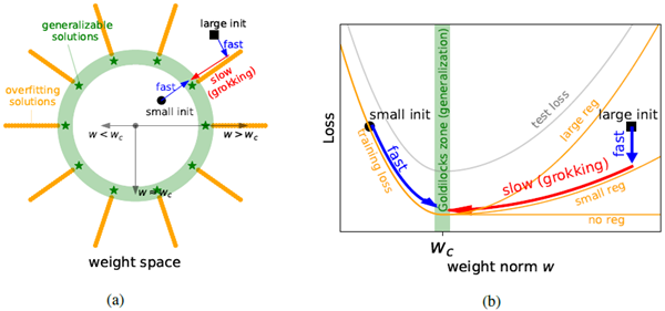
Figure 1: (a) \(w: L_2\) norm of model weights. Generalizing solutions (green stars) are concentrated around a sphere in the weight space where \(w \approx w_c\) (green). Overfitting solutions (orange) populate the \(w \overset{\gt}{\sim} w_c\) region. (b) The training loss (orange) and test loss (gray) have the shape of L and U,
respectively. Their mismatch in the \(w \gt w_c\) region leads to fast-slow dynamics, resulting in grokking.
図1: (a) モデルの重みの \(w: L_2\) ノルム。一般化解(緑の星印)は、重み空間において \(w \approx w_c\)(緑)の球面付近に集中している。過学習解(オレンジ)は \(w \overset{\gt}{\sim} w_c\) 領域を占めている。(b) 訓練損失(オレンジ)とテスト損失(灰色)は、それぞれL字型とU字型の形状をしている。\(w \gt w_c\) 領域におけるそれらの不一致は、高速・低速ダイナミクスにつながり、結果としてグロッキングを引き起こす。
-
A2 Yes. Indeed, we demonstrate grokking for a wide range of machine learning tasks in Section 4, including image classification, sentiment analysis and molecule property prediction. Grokking signals observed for these tasks are usually less dramatic than for algorithmic datasets, which we attribute to representation learning in Section 5.
はい。実際、第4章では、画像分類、感情分析、分子特性予測など、幅広い機械学習タスクにおけるGrokkingの有効性を示しました。これらのタスクで観測されるGrokkingシグナルは、アルゴリズムデータセットの場合ほど劇的ではありません。これは、第5章で表現学習によるものだと考えています。
Partial answers to Q1 are provided in recent studies: Liu et al. (2022) attribute grokking to the slow formation of good representations, Thilak et al. (2022) attempts to link grokking to the slingshot mechanism of adaptive optimizers, and Barak et al. (2022) uses Fourier gap to describe hidden progress. This paper aims to understand grokking through the lens of neural loss landscapes. Our landscape analysis is able to explain many aspects of grokking: data size dependence, weight decay dependence, emergence of representations, etc.
Q1に対する部分的な回答は、最近の研究で示されています。Liu et al. (2022) は、グロッキングを良好な表現の緩やかな形成に帰し、Thilak et al. (2022) はグロッキングを適応型最適化器のスリングショットメカニズムと関連付け、Barak et al. (2022) はフーリエギャップを用いて隠れた進歩を記述しています。本論文は、ニューラル損失ランドスケープの観点からグロッキングを理解することを目指しています。ランドスケープ分析は、データサイズ依存性、重み減衰依存性、表現の創発など、グロッキングの多くの側面を説明することができます。
The paper is organized as follows: In Section 2, we review background on generalization, and introduce the LU mechanism. In Section 3, we show how the LU mechanism leads to grokking for a toy teacher-student setup. In Section 4, we show that the intuition gained from the toy problem can transfer to realistic datasets (MNIST, IMDb reviews and QM9), for which we also observe grokking, although in a slightly non-standard setup where it is relatively weak. In Section 5, we discuss why grokking is more dramatic for algorithmic datasets than on others (e.g., MNIST), by comparing their loss landscapes. As a byproduct, we find that training with constrained weight norm can almost eliminate grokking. We review related work in Section 6 and summarize our conclusions in Section 7. Code is available at https://github.com/KindXiaoming/Omnigrok.
この論文は次のように構成されています。第2節では、一般化の背景をレビューし、LUメカニズムを紹介します。第3節では、LUメカニズムがおもちゃの教師と生徒の設定でどのようにグロッキングにつながるかを示します。第4節では、おもちゃの問題から得られた直感が現実的なデータセット(MNIST、IMDbレビュー、QM9)に転用できることを示します。これらのデータセットでもグロッキングが見られますが、やや非標準的な設定では比較的弱いです。第5節では、アルゴリズムデータセットの方が他のデータセット(MNISTなど)よりもグロッキングがより劇的である理由を、それらの損失ランドスケープを比較することにより説明します。副産物として、制約付き重みノルムを使用したトレーニングによってグロッキングをほぼ排除できることがわかります。第6節では関連作業をレビューし、第7節で結論をまとめます。コードはhttps://github.com/KindXiaoming/Omnigrokで入手できます。
2 THE LU MECHANISM FOR GROKKING グロッキングのためのLUメカニズム
Weight norm and reduced loss Letting \(\mathbf{w}\) denote the weights of a model, any function \(f(\mathbf{w})\) (e.g, train/test loss/accuracy) depends on both the weight norm \(w\equiv||w||_2\) and the angular direction \(\hat{\mathbf{w}}\equiv \mathbf{w}/w\). Similar to (Fort and Scherlis, 2019), we define a reduced function \(\tilde{f}(w)\) by minimizing training loss \(l_{train}(\mathbf{w})\) over angular directions, i.e.,
重みノルムと縮約損失 モデルの重みを \(\mathbf{w}\) とすると、任意の関数 \(f(\mathbf{w})\) (例えば、訓練/テストの損失/精度) は、重みノルム \(w\equiv||w||_2\) と角度方向 \(\hat{\mathbf{w}}\equiv \mathbf{w}/w\) の両方に依存します。 (Fort and Scherlis, 2019) と同様に、角度方向にわたって訓練損失 \(l_{train}(\mathbf{w})\) を最小化することで縮約関数 \(\tilde{f}(w)\) を定義します。つまり、
\[
\tilde{f}(w)\equiv f(\mathbf{w}^*(w)),\quad \text{where }\mathbf{w}^*(w)\equiv \text{arg}\min\limits_{||\mathbf{w}||_2} l_{train}(\mathbf{w}) \tag{1}
\]
In practice, we perform the constrained minimization by rescaling the model weights back to their original norm after each unconstrained optimization step. We will see that this reduced 1D loss landscape, which is easy to visualize, captures important features related to grokking. Throughout the paper, our model is initialized by multiplying a factor \(α\equiv w/w_0\) to the standard initialization 1,
where \(w_0\) and \(w\) are the weight norm of the network before and after multiplying \(α\).
実際には、制約なしの最適化ステップごとにモデルの重みを元のノルムに再スケーリングすることで、制約付き最小化を実行します。この縮小された1次元損失ランドスケープは視覚化が容易で、グロッキングに関連する重要な特徴を捉えていることがわかります。本論文全体を通して、モデルは標準的な初期化値1に係数\(α\equiv w/w_0\)を乗じて初期化されます。
ここで、\(w_0\)と\(w\)は、\(α\)を乗じる前と乗じた後のネットワークの重みノルムです。
1
The standard initialization means the default one in PyTorch.
標準の初期化は、PyTorch のデフォルトの初期化を意味します。
LU mechanism Although the loss landscapes of neural networks are nonlinear, (Fort and Scherlis, 2019) reveal a simple landscape picture: There is a spherical shell in the weight space (the "Goldilocks" zone), where generalization is better than outside this zone. We illustrate the Goldilocks
zone as the green area with average radius \(w_c\) in Figure 1a; the green stars are the generalizing solutions. The test loss is thus higher either both when \(w \gt w_c\) and \(w \lt w_c\), forming a U-shape
against \(w\) in Figure 1b (gray curve). By contrast, the training loss has an L-shape against weight
norm 2. There are many solutions which overfit training data for \(w \gt w_c\), but high training losses are incurred for \(w \lt w_c\). This corresponds to the L-shaped curve seen in Figure 1b (orange curve,
no regularization). In summary, the (reduced) training loss and test loss are L-shaped and U-shaped against weight norm, respectively, which we will refer to as the LU mechanism throughout the paper.
LUメカニズム ニューラルネットワークの損失ランドスケープは非線形ですが、(Fort and Scherlis, 2019) は単純なランドスケープ像を示しています。重み空間(「ゴルディロックス」ゾーン)には球殻があり、このゾーン外よりも汎化性能が優れています。図1aでは、ゴルディロックスゾーンを平均半径 \(w_c\) の緑色の領域として示しています。緑色の星印は汎化解です。したがって、テスト損失は \(w \gt w_c\) と \(w \lt w_c\) の両方で高くなり、図1b(灰色の曲線)では \(w\) に対してU字型を形成します。対照的に、トレーニング損失は重みノルム 2 に対してL字型になります。\(w \gt w_c\) のトレーニングデータに過剰適合する解は多数存在しますが、\(w \lt w_c\) では高いトレーニング損失が発生します。これは図1b(オレンジ色の曲線、正則化なし)に示されているL字型の曲線に対応します。要約すると、(縮小された)トレーニング損失とテスト損失は、重みノルムに対してそれぞれL字型とU字型であり、本稿ではこれをLUメカニズムと呼ぶことにします。
2\(l_{train}(w)\) is non-increasing: One can always construct a larger network by adding useless non-zero weights to a smaller network, without changing the functionality of the model.
\(l_{train}(w)\) は非増加です。モデルの機能を変えずに、小さなネットワークに無駄な非ゼロの重みを追加することで、より大きなネットワークを構築することができます。
It is well known in statistics that generalization error has a "U" shape against model capacity, which is usually attributed to the bias-variance trade-off. Although this common wisdom was challenged by the observation of double descent (Nakkiran et al., 2021), the "U" curve can be recovered from a double descent simply by changing the x-axis from the number of model parameters N to the 2-norm of model parameters \(w \equiv ||w||_2\) (Ng and Ma, 2022). Although the LU mechanism may remind
readers of related phenomena (Schoenholz et al., 2016; Yang and Schoenholz, 2017; Nakkiran et al., 2021), their setups are not exactly the same as ours. More importantly, our focus and contribution is to understand grokking, a brand new generalization puzzle.
統計学では、汎化誤差がモデル能力に対して「U」字型になることがよく知られており、これは通常、バイアスと分散のトレードオフに起因するとされています。この常識は二重降下現象の観察によって疑問視されましたが(Nakkiran et al., 2021)、二重降下現象から「U」曲線を復元するには、x軸をモデルパラメータの数Nからモデルパラメータの2次元ノルム\(w \equiv ||w||_2\)に変更するだけで済みます(Ng and Ma, 2022)。LUメカニズムは、読者に関連現象(Schoenholz et al., 2016; Yang and Schoenholz, 2017; Nakkiran et al., 2021)を想起させるかもしれませんが、それらの設定は私たちのものと全く同じではありません。さらに重要なのは、私たちの焦点と貢献は、全く新しい汎化パズルであるグロッキングを理解することです。
Grokking dynamics We identify the "LU mechanism" as the cause of grokking. If the weight norm is initialized to be large (e.g., the black square in the \(w \gt w_c\) region), the model first quickly moves to a
nearby overfitting solution by minimizing the training loss. Without any regularization, the model will stay where it is, because the gradient of the training loss is almost zero along the valley of overfitting solutions, so generalization does not happen. Fortunately, there are usually explicit and/or implicit
regularizations that can drive the weight vector towards the Goldilocks zone \(w \approx w_c\). When the
regularization magnitude is non-zero but small, the radial motion can be (arbitrarily) slow. If weight
decay is the only source of regularization, and training loss is negligible after overfitting, then weight
decay \(γ\) causes \(w(t) \approx \exp(-γt)w_0\), when \(w_0 \gt w_c\), so it takes time \(t \approx \ln(w_0/w_c)/γ\propto γ^{-1}\) to
generalize. A small \(γ\) results in a huge generalization delay (i.e., grokking). The dependence on
regularization magnitudes is illustrated in Figure 1b: no generalization at all happens for \(γ= 0\),
small \(γ\) leads to slow generalization (grokking), and large \(γ\) leads to faster generalization 3. The
above analysis only applies to large initializations \(w \gt w_c\). Small initializations \(w \lt w_c\) can always
generalize fast 4, regardless of regularization.
グロッキングダイナミクス グロッキングの原因として「LUメカニズム」を特定しました。重みノルムが大きく初期化されている場合(例えば、\(w \gt w_c\)領域の黒い四角)、モデルはまず訓練損失を最小化することで近くの過適合解に素早く移動します。正則化を行わない場合、訓練損失の勾配は過適合解の谷間に沿ってほぼゼロであるため、モデルは現状のままで、汎化は起こりません。幸いなことに、通常は明示的または暗黙的な正則化によって重みベクトルをゴルディロックスゾーン\(w \approx w_c\)に近づけることができます。正則化の程度がゼロではないが小さい場合、放射状の移動は(任意に)遅くなる可能性があります。重みの減衰が正則化の唯一の要因であり、過学習後の訓練損失が無視できる場合、重みの減衰 \(γ\) により \(w_0 \gt w_c\) のときに \(w(t) \approx \exp(-γt)w_0\) が生じるため、汎化には \(t \approx \ln(w_0/w_c)/γ\propto γ^{-1}\) の時間がかかります。\(γ\) が小さいと、汎化(つまり、グロッキング)の遅延が大きくなります。正則化の程度への依存性は図 1b に示されています。\(γ= 0\) の場合、汎化は全く起こりません。\(γ\) が小さいと、汎化(グロッキング)が遅くなり、\(γ\) が大きいと、汎化が速くなります 3。
上記の分析は、初期化値が大きい \(w \gt w_c\) にのみ適用されます。小さな初期化 \(w \lt w_c\) は、正規化の有無にかかわらず、常に高速 4 を一般化できます。
3 \(γ\) should not be too large, otherwise it will bring the weights to a trivial solution \(\mathbf{w} = \mathbf{0}\)
\(γ\) は大きすぎてはいけません。大きすぎると重みが単純な解 \(\mathbf{w} = \mathbf{0}\) になってしまいます。
4 \(w\) should not be too small to harm optimization.
\(w\) は最適化に悪影響を与えるほど小さくなってはいけません。
Why isn’t grokking commonly observed ? The standard initialization schemes typically initialize
\(w\) no larger than \(w_c\). However, if we increase initialization scales (explicitly or implicitly), grokking
can appear. In Section 3 and 4, we find that explicitly increasing initialization weight norm can induce grokking. In Section 5, we argue for algorithmic datasets because (shown in Figure 6d)
なぜグロッキングは一般的に観察されないのか? 標準的な初期化スキームでは通常、\(w\) が \(w_c\) より大きくならないように初期化されます。しかし、初期化スケールを(明示的または暗黙的に)大きくすると、グロッキングが
発生する可能性があります。第3章と第4章では、初期化重みノルムを明示的に大きくするとグロッキングが誘発される可能性があることを示します。第5章では、アルゴリズムデータセットの利点について論じます。その理由は(図6dに示すように)
\[
w_c(\text{悪い表現}) \gt w_c(\text{良い表現}) \tag{2}
\]
i.e., a proper initialization for a bad representation is effectively too large for a good representation,
leading to grokking. Take the addition (base p) for example: with the good (linear) representation
or a bad (random) representation, the decoder needs to learn to classify \(O(p)\) or \(O(p^2)\) examples, respectively.
つまり、悪い表現に対する適切な初期化は、良い表現に対しては事実上大きすぎるため、
グロッキング(grokking)につながります。例えば、加算(基数p)を考えてみましょう。良い(線形)表現の場合、
デコーダーはそれぞれ\(O(p)\)または\(O(p^2)\)の例を分類することを学習する必要があります。
3 GROKKING FOR A TEACHER-STUDENT SETUP 教師-生徒セットアップのためのグロッキング
To illustrate how the LU mechanism results in grokking, we employ a toy teacher-student setup. The teacher and the student share the same architecture (a 5-100-100-5 MLP with tanh activation), but are initialized with different seeds. The student network is initialized with the standard initialization
(the default one in PyTorch) but each weight is rescaled by the same factor \(α\equiv w/w_0\), where \(w_0\) and \(w\) are the weight norm of the student network before and after rescaling. The teacher network is initialized standardly, i.e., \(α_{teacher} = 1\). Inputs and outputs have dimensions \(d_{in}= 5\) and \(d_{out}= 5\), respectively. We generate \(N_{train} = 100\) training and \(N_{test}= 100\) test samples by first drawing inputs from the standard Gaussian distribution \(N(0, \mathbf{I}_{d_{in}×d_{in}})\), and then feed the input data to the teacher to generate output labels. The student network is trained with the Adam optimizer (learning rate
3×10⁻⁴) for 105 steps.
LUメカニズムがどのようにグロッキングをもたらすかを説明するために、模擬的な教師-生徒ネットワーク構成を採用する。教師ネットワークと生徒ネットワークは同じアーキテクチャ(tanh活性化を伴う5-100-100-5 MLP)を共有するが、異なるシード値で初期化する。生徒ネットワークは標準的な初期化(PyTorchのデフォルト)で初期化されるが、各重みは同じ係数 \(α\equiv w/w_0\) で再スケーリングされる。ここで、\(w_0\) と \(w\) は、再スケーリング前後の生徒ネットワークの重みノルムである。教師ネットワークは標準的な初期化、すなわち \(α_{teacher} = 1\) で初期化される。入力と出力の次元はそれぞれ \(d_{in}= 5\) と \(d_{out}= 5\) である。まず標準ガウス分布 \(N(0, \mathbf{I}_{d_{in}×d_{in}})\) から入力データを抽出し、\(N_{train} = 100\) 個のトレーニングサンプルと \(N_{test} = 100\) 個のテストサンプルを生成します。次に、入力データを教師に与えて出力ラベルを生成します。生徒ネットワークは、Adam オプティマイザー(学習率
3×10⁻⁴)を用いて 105 ステップで学習されます。
LU landscapes Firstly, we compute the reduced losses by minimizing the training loss (excluding weight decay) while constraining the weight norm of the student network to be constant. We treat the converging point after training as the global minimum on the spherical surface, which explicitly defines the reduced losses \(\tilde{l}_{train}(α)\) and \(\tilde{l}_{test}(α)\). As shown in Figure 2a, \(\tilde{l}_{test}(α)\) first decreases and then increases as α increases, displaying a U-shape with a minimum at \(α\approx 1\). By contrast, \(\tilde{l}_{train}(α)\) decreases when \(α \lt 1\) and remains flat near zero when \(α \geq 1\),forming an L-shape. When weight decay \(γ\) is present, the training landscape becomes \(\tilde{l}_{train}(α, γ) = \tilde{l}_{train}(α) + γα^2C^2\) where \(C\) is the average parameter magnitude determined by the standard initialization.
LU ランドスケープ まず、学習ネットワークの重みノルムを一定に制約しながら、学習損失(重みの減衰を除く)を最小化することで、縮減損失を計算します。学習後の収束点を球面上の大域的最小値として扱い、縮減損失 \(\tilde{l}_{train}(α)\) と \(\tilde{l}_{test}(α)\) を明示的に定義します。図 2a に示すように、\(\tilde{l}_{test}(α)\) は最初減少し、その後 \(α\) が増加するにつれて増加して、\(α\approx 1\) で最小値となる U 字型を示します。対照的に、\(\tilde{l}_{train}(α)\) は \(α \lt 1\) のときに減少し、\(α \geq 1\) のときはゼロ付近で平坦となり、L 字型を形成します。重みの減少 \(γ\) が存在する場合、トレーニング ランドスケープは \(\tilde{l}_{train}(α, γ) = \tilde{l}_{train}(α) + γα^2C^2\) になります。ここで、\(C\) は標準の初期化によって決定される平均パラメーターの大きさです。
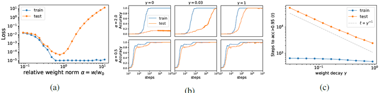
Figure 2: Teacher-student setup. : student initialization scale, : weight decay. (a) The reduced training loss and test loss have the shape of "L" and "U", respectively. (b) Top row: large initialization (\(α = 2.0\)) can demonstrate no generalization (no reg), grokking (small reg) and fast generalization (large reg). Bottom: small initialization (\(α = 0.5\)) always generalizes fast, regardless of weight deacy. (c) \(α = 2\). The steps to overfitting is independent of weight decay, while the steps to generalization scale inversely with the weight decay.
図2:教師と生徒のセットアップ。 : 生徒の初期化スケール、 : 重みの減衰。(a) 縮小されたトレーニング損失とテスト損失は、それぞれ「L」と「U」の形状をしています。(b) 上段:大きな初期化(α = 2.0)では、汎化なし(regなし)、グロッキング(小さなreg)、高速汎化(大きなreg)が見られます。下段:小さな初期化(α = 0.5)では、重みの減衰に関係なく、常に高速汎化が見られます。(c) α = 2。過学習へのステップは重みの減衰とは無関係ですが、汎化へのステップは重みの減衰に反比例します。
Training dynamics Our problem is a regression task, but we can imitate the behavior of a classifica-tion task by manually setting a threshold \(θ= 0.01\) and defining a sample to be correctly “classified" if the prediction error is less than . We study the dynamics of training and test accuracy. We run experiments with two initializations \(α= 0.5\) (small) and \(α= 2.0\) (large), and three weight decays \(γ= 0\) (no reg),\(γ= 0.03\) (small reg) and \(γ= 1\) (large reg). As shown in Figure 2b (bottom), small initialization runs always generalize fast regardless of regularization. Large initialization runs (top) depended on weight decay: no regularization fails to generalize, small regularization generalizes slowly (grokking), while large regularization generalizes faster.
トレーニング ダイナミクス 今回の問題は回帰タスクですが、しきい値 \(θ= 0.01\) を手動で設定し、予測誤差が 未満の場合にサンプルが正しく「分類」されるように定義することで、分類タスクの動作を模倣できます。トレーニングとテストの精度のダイナミクスを調べます。2 つの初期化 \(α= 0.5\) (小さい) と \(α= 2.0\) (大きい)、および 3 つの重みの減衰 \(γ= 0\) (正規化なし)、\(γ= 0.03\) (小さい正規化)、および \(γ= 1\) (大きい正規化) を使用して実験を実行します。図 2b (下) に示すように、小さい初期化の実行では、正規化に関係なく、常に高速に一般化されます。大きい初期化の実行 (上) は重みの減衰に依存していました。正規化なしだと一般化に失敗し、小さい正規化では一般化が遅くなります (grokking)。一方、大きい正規化では一般化が高速になります。
For the large initialization \(α= 2.0\), we do a finer sweep of \(γ\) in [0.03,1]. We compute the number of steps and weight norm w when training or test accuracy reaches 95%. As shown in Figure 2c, the time (number of steps) to reach 95% training accuracy is independent of weight decay \(γ\), while the time to reach 95% test accuracy is inversely proportional to the weight decay, as we derived above for the LU mechanism.
大きな初期化\(α= 2.0\)の場合、\(γ\)を[0.03,1]の範囲でより細かく掃引します。訓練またはテストの精度が95%に達したときのステップ数と重みノルムwを計算します。図2cに示すように、訓練精度95%に達するまでの時間(ステップ数)は重みの減衰\(γ\)とは独立していますが、テスト精度95%に達するまでの時間は、LUメカニズムについて上で導出したように、重みの減衰に反比例します。
4 OMNIGROK: GROKKING FOR MORE INTERESTING TASKS OMNIGROK: もっと面白いタスクを探そう
We now analyze loss landscapes and search for grokking for several more interesting datasets, and see that the insights obtained from our toy model can transfer to these datasets. We report the main results here, with experiment details included in Appendix A.
我々は現在、損失ランドスケープを分析し、さらに興味深いデータセットのグロッキングを探索しています。その結果、我々のトイモデルから得られた知見がこれらのデータセットにも適用できることがわかりました。主な結果をここに報告し、実験の詳細は付録Aに記載しています。
Image classification We visualize loss landscapes of MNIST (Deng, 2012) to verify the LU mech-anism, and study the dependence on training data size. Similar to the teacher-student case, we reduce losses and errors (one minus accuracy) to two variables (weight norm w and data size N) by minimizing over angular directions of weights, i.e.,
画像分類 LUメカニズムを検証するため、MNIST (Deng, 2012) の損失ランドスケープを可視化し、学習データサイズへの依存性を調べた。教師-生徒の場合と同様に、重みの角度方向を最小化することで、損失と誤差(1から精度を引いたもの)を2つの変数(重みノルムwとデータサイズN)に減らす。すなわち、
\[
\tilde{l}_{train}(w,N)\equiv l_{train}(\mathbf{w}^*,N),\quad \tilde{l}_{test}(w,N)\equiv l_{test}(\mathbf{w}^*,N),\quad \mathbf{w}^*(w,N)\equiv \text{arg}\min\limits_{||\mathbf{w}||_2=w} l_{train}(\mathbf{w},N) \tag{3}
\]
shown in Figure 3 (a)(b). The reduced loss landscape reveals three things: (1) Larger initializations lead to grokking. Point A in Figure 3 corresponds to the standard initialization (\(α=1\)), which has low training and test errors, hence no grokking. When increasing the weight norm from A to B, training error is seen to remain low while test error rises. To generalize, implicit or explicit regularization such as weight decay then brings the weight norm down, leading to delayed generalization (grokking) if regularization is small. (2) Larger datasets lead to de-grokking. Comparing B and C in Figure 3, C is seen to have larger training size than B and lower test error. Larger data size \(N\) makes the Goldilocks zone broader, reducing or eliminating grokking even for large weight initializations. (3) Critical data size can be defined. As reported in (Power et al., 2022; Liu et al., 2022), we see that there exists a critical training set size below which generalization is impossible. The effective theory analysis in (Liu et al., 2022) only applies to algorithmic datasets, but not to other datasets with unknown optimal representations. The loss landscape analysis presented is this work can apply to all supervised-learning tasks. As shown in Figure 3 (b), the contours of constant test error are thumb-like, and the tip of the thumb determines the minimum amount of data required for generalization.
図3(a)(b)に示されています。損失ランドスケープの縮小から、次の3つのことがわかります。(1) 初期化が大きくなるほど、グロッキングが発生します。図3のポイントAは、トレーニング エラーとテスト エラーが低いため、グロッキングが発生しない標準的な初期化(\(α=1\))に対応します。重みノルムをAからBに増やすと、トレーニング エラーは低いままですが、テスト エラーが増加することがわかります。一般化するには、重みの減衰などの暗黙的または明示的な正則化によって重みノルムが低下し、正則化が小さい場合は一般化(グロッキング)が遅れます。(2) データセットが大きいほど、グロッキングが解消されます。図3のBとCを比較すると、CはBよりもトレーニング サイズが大きく、テスト エラーが低いことがわかります。データ サイズ \(N\) が大きいほど、ゴルディロックス ゾーンが広くなり、重みの初期化が大きい場合でもグロッキングが削減または排除されます。(3) 臨界データ サイズを定義できます。 (Power et al., 2022; Liu et al., 2022) で報告されているように、訓練セットのサイズが臨界値に達し、それ以下では汎化が不可能になることがわかります。(Liu et al., 2022) の有効理論分析はアルゴリズムデータセットにのみ適用され、最適な表現が不明な他のデータセットには適用されません。本研究で提示されている損失ランドスケープ分析は、すべての教師あり学習タスクに適用できます。図3 (b) に示すように、一定テスト誤差の等高線は親指のような形をしており、親指の先端が汎化に必要な最小データ量を決定します。
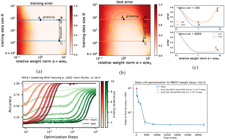
Figure 3: MNIST. (a) reduced training error, (b) reduced test error. Comparing A and B: larger weight norm makes learning grok (delay generalization). Comparing B and C: a larger training data size makes learning de-grok (speed up generalization). (c) "LU" holds truer for smaller data. (d) Accuracy curves for MNIST in the setting where we observe grokking. (e) Time to generalize as a function of training set size N.
図3:MNIST。(a) 学習エラーの減少、(b) テストエラーの減少。AとBの比較:重みノルムが大きいほど学習がグロックしやすくなる(一般化が遅れる)。BとCの比較:学習データのサイズが大きいほど学習がグロックしやすくなる(一般化が加速する)。(c) LUはデータサイズが小さいほどより真実である。(d) グロッキングが見られる設定におけるMNISTの精度曲線。(e) 学習セットサイズNの関数としての一般化時間。
Guided by the landscape analysis, we make two nonstandard decisions to induce grokking on MNIST: (1) we reduce the size of the training set from 60k to 1k samples (by taking a random subset) and (2) we increase the scale of the weight initialization distribution (by multiplying the initial weights, sampled with Kaiming uniform initialization, by a constant \(α \gt 1\)). With these modifications to the training set size and initialization scale, we train a depth-3 width-200 MLP with ReLU activations with the AdamW optimizer using MSE loss with one-hot targets. We find that the network quickly fits the training set, and test accuracy improves much later, as shown in Figure 3d, just as in the stereotypical grokking learning first observed in algorithmic datasets. Figure 3e shows the effect of training set size on time to generalization for MNIST. We find a result similar to what (Power et al., 2022) observed, namely that generalization time increases rapidly once one approaches a certain critical data set size. We also include the learning phase diagram in Appendix ??.
ランドスケープ分析に基づき、MNIST のグロッキングを誘導するために、2 つの非標準的な決定を下します。(1) トレーニング セットのサイズを 60k サンプルから 1k サンプルに減らす (ランダムなサブセットを取得することにより)、(2) 重みの初期化分布のスケールを増やす (Kaiming 均一初期化でサンプリングされた初期の重みに定数 \(α \gt 1\) を掛けることにより)。トレーニング セットのサイズと初期化スケールをこのように変更し、深さ 3、幅 200 の MLP を、ReLU アクティベーションを使用して AdamW オプティマイザーでトレーニングします。これは、ワンホット ターゲットで MSE 損失を使用します。ネットワークはトレーニング セットにすばやく適合し、図 3d に示すように、アルゴリズム データ セットで最初に観察された典型的なグロッキング学習と同様に、テスト精度がかなり後で向上することがわかります。図 3e は、MNIST の一般化までの時間に対するトレーニング セットのサイズの影響を示しています。 (Power et al., 2022) の観察結果と類似した結果、すなわち、ある臨界データセットサイズに近づくと、汎化時間が急激に増加することがわかりました。学習フェーズダイアグラムも付録 ?? に掲載しています。
Sentiment analysis of text We look for grokking using LSTMs (Hochreiter and Schmidhuber, 1997) for IMDb dataset (Maas et al., 2011). Similar to Eq. (3), we reduce training and test losses to depend on only the weight norm w and data size N. We show the reduced training and test error in Figure 4
(a)(b). For large data size say the full dataset, training and test errors have similar "U" shapes 5, so one cannot create grokking via the "LU" mechanism. For small data size, say 1k, however, the mismatch between training and test errors makes it possible to create grokking via large initializations. In
Figure 4 (c), we initialize weights larger (\(α = 6\)) with weight decay 1, overfitting is complete within
102 steps, but generalization does not start until around 103 steps. Note that the generalization "jump" is not as sharp as on algorithmic datasets (Power et al., 2022) or MNIST, but at least generalization is delayed here. By contrast, if we use the standard initialization (\(α = 1\9) with no weight decay, generalization happens early on during training, and does not improve much after overfitting.
テキストの感情分析 IMDbデータセット(Maas et al., 2011)に対して、LSTM(Hochreiter and Schmidhuber, 1997)を用いてグロッキングを試行します。式(3)と同様に、学習とテストの損失を重みノルムwとデータサイズNのみに依存するように削減します。削減された学習とテストの誤差を図4
(a)(b)に示します。データサイズが大きい場合(例えばデータセット全体)、学習とテストの誤差は類似した「U」字型5となるため、「LU」メカニズムを用いてグロッキングを生成することはできません。しかし、データサイズが小さい場合(例えば1k)は、学習とテストの誤差の不一致により、大きな初期化によってグロッキングを生成することが可能になります。
図4 (c)では、重みをより大きな値(\(α = 6\))に重み減衰1で初期化しています。過学習は102ステップ以内に完了しますが、汎化は103ステップ程度まで開始されません。汎化の「飛躍」はアルゴリズムデータセット(Power et al., 2022)やMNISTほど急激ではありませんが、少なくともここでは汎化が遅れています。対照的に、重み減衰のない標準的な初期化(\(α = 1\9))を使用した場合、汎化はトレーニングの早い段階で起こり、過学習後もそれほど改善されません。
5
In principle, reduced training losses should be non-increasing ("L"), but optimization issues may occur for too large initializations (Schoenholz et al., 2016).
原則として、トレーニング損失の削減は非増加(「L」)になるはずですが、初期化が大きすぎると最適化の問題が発生する可能性があります(Schoenholz 他、2016)。
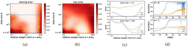
Figure 4: We use an LSTM to predict IMDb reviews. (a) training error; (b) test error; (c) reduced losses for data size 1k (top) and 50k (bottom); (d) With 1k data, a (weak) grokking signal is observed for large initializations (\(α= 6\)), while no grokking is observed for standard initializations (\(α= 1\)).
図 4: LSTM を使用して IMDb のレビューを予測します。(a) トレーニング エラー、(b) テスト エラー、(c) データ サイズ 1k (上) と 50k (下) の損失の削減、(d) 1k データの場合、大規模な初期化 (\(α= 6\)) では (弱い) グロッキング信号が観測されますが、標準的な初期化 (\(α= 1\)) ではグロッキングは観測されません。
Molecules We search for grokking using the graph convolutional neural network (GCNN) for QM9 dataset (Ramakrishnan et al., 2014). Similar to Eq. (3), we define the reduced training/test losses, which are only dependent on weight norm \(w\) and data size N. As shown in Figure 5(a)(b), when data size is large, training and test losses have similar "U" shapes, hence grokking is impossible via the "LU mechanism". When data size is small, training and test losses mismatch somewhere in the region
\(α= w=w_0 \gt 1\), making grokking possible. Indeed, shown in Figure 5(d), there is a sharp drop in test
loss around 104 steps if initialization is 3 times larger than standard, while standard initialization does not lead to grokking. Note that zero weight decay is applied in both cases, implying the existence of implicit regularizations.
分子 QM9データセット(Ramakrishnan et al., 2014)に対して、グラフ畳み込みニューラルネットワーク(GCNN)を用いてグロッキングを探索する。式(3)と同様に、重みノルム \(w\) とデータサイズ N のみに依存する、縮減されたトレーニング/テスト損失を定義する。図5(a)(b)に示すように、データサイズが大きい場合、トレーニング損失とテスト損失は類似した「U」字型になるため、「LUメカニズム」によるグロッキングは不可能である。データサイズが小さい場合、トレーニング損失とテスト損失は領域\(α= w=w_0 \gt 1\) のどこかで不一致となり、グロッキングが可能となる。実際、図5(d)に示すように、初期化が標準の3倍の場合、104ステップ付近でテスト損失が急激に減少するが、標準的な初期化ではグロッキングは達成されない。どちらの場合もゼロ重み減衰が適用され、暗黙的な正規化が存在することを意味することに注意してください。
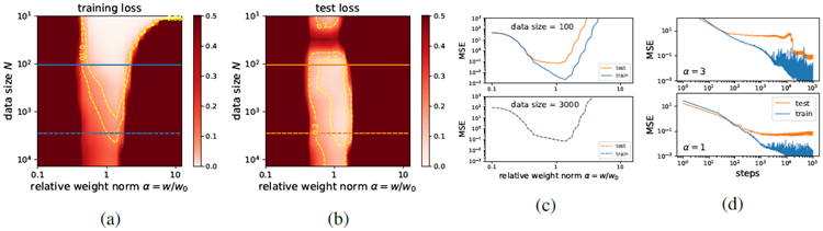
Figure 5: We use a GCNN to predict isotropic polarizability of molecules in the QM9 dataset. (a) training loss; (b) test loss; (c) reduced losses for data size 100 (top) and 3000 (bottom); (d) with 200 training samples, grokking is observed for large initialization (\(α = 3\)), while no grokking is observed for standard initializations (\(α = 1\)).
図 5: GCNN を使用して、QM9 データセット内の分子の等方性分極率を予測します。(a) トレーニング損失、(b) テスト損失、(c) データ サイズ 100 (上) および 3000 (下) の損失の削減、(d) トレーニング サンプル数が 200 の場合、大規模な初期化 (\(α = 3\)) ではグロッキングが観察されますが、標準的な初期化 (\(α = 1\)) ではグロッキングは観察されません。
5 REPRESENTATION IS KEY TO GROKKING 表現はグロッキングへの鍵
In Section 4, we showed that increasing initialization scales can make grokking happen for standard ML tasks. However, this seems a bit artificial and does not explain why standard initialization leads to grokking on algorithmic datasets, but not on standard ML datasets, say MNIST. The key difference is how much the task relies on representation learning. For the MNIST dataset, the quality of representation determines whether the test accuracy is 95% or 100%; by constrast in algorithmic datasets, the quality of representation determines whether test accuracy is random guess (bad representation) or 100% (good representation). So overfitting (under a bad representation) has a more dramatic effect on algorithmic datasets, i.e., the model weights increase quickly during overfitting but test accuracy remains low. During overfitting, model weight norm is much larger than at initialization, but then drops below the initialization norm when the model generalizes, shown in Figure 7a, and also observed by (Nanda et al., 2023). As a byproduct, we are able to eliminate grokking by constraining the model on a small weight norm sphere, shown in Figure 7b.
セクション 4 では、初期化スケールを増やすと標準的な ML タスクでグロッキングが起こる可能性があることを示しました。しかし、これは少し不自然で、標準的な初期化がアルゴリズム データセットではグロッキングにつながるのに、MNIST などの標準的な ML データセットではつながらない理由を説明していません。重要な違いは、タスクが表現学習にどの程度依存しているかです。MNIST データセットの場合、表現の品質によってテスト精度が 95% になるか 100% になるかが決まります。対照的に、アルゴリズム データセットでは、表現の品質によってテスト精度がランダム推測 (悪い表現) になるか 100% (良い表現) になるかが決まります。そのため、(悪い表現の下での) 過学習はアルゴリズム データセットにより劇的な影響を及ぼします。つまり、過学習中はモデルの重みが急速に増加しますが、テスト精度は低いままです。過学習中、モデルの重みのノルムは初期化時よりもはるかに大きくなりますが、モデルが一般化すると初期化ノルムを下回ります。これは図 7a に示されており、(Nanda et al., 2023) でも観察されています。副産物として、図 7b に示すように、モデルを小さな重みノルム球に制約することによって、グロッキングを排除することができます。
In the following, we will compare algorithmic datasets (Section 5.1) to MNIST (Section 5.2). We show how their loss landscapes depend on representations differently, and how the difference leads to different outcomes (grokking or not).
以下では、アルゴリズムデータセット(セクション5.1)とMNIST(セクション5.2)を比較します。これらのデータセットの損失ランドスケープが表現方法によってどのように異なるか、そしてその違いが結果(グロッキングの有無)にどのように影響するかを示します。
5.1 ALGORITHMIC DATASETS アルゴリズムデータセット
Setup We take the toy addition setup in (Liu et al., 2022), where each input digit \(0 \leq i \leq p - 1\)(output label \(0 \leq k \leq 2(q - 1)\)) is embedded as a vector \(\mathbf{E}_i(\mathbf{Y}_k)\). A decoder MLP is employed to predict \(\mathbf{Y}_k = Dec(\mathbf{E}_i + \mathbf{E}_j) (k = i + j)\). In the setup of grokking, both the decoder and the input representations \(\mathbf{R}\equiv \{\mathbf{E}_i\}\) are trainable, with learning rates \(η_D\) and \(η_R\), respectively; in the setup of
landscape analysis, only decoder is trainable, as we explain below. Training and test losses depend on three factors: (i) representation \(\mathbf{R}\), (ii) weight norm w and (iii) weight direction w. As in previous sections, we can optimize w by minimizing the training loss on constant weight norm spheres. We further reduce the high-dimensional representations to 1D by interpolating in a particular direction:
セットアップ (Liu et al., 2022) のおもちゃの加算セットアップを採用します。ここで、各入力数字 \(0 \leq i \leq p - 1\)(出力ラベル \(0 \leq k \leq 2(q - 1)\)) はベクトル \(\mathbf{E}_i(\mathbf{Y}_k)\) として埋め込まれます。デコーダー MLP を使用して、\(\mathbf{Y}_k = Dec(\mathbf{E}_i + \mathbf{E}_j) (k = i + j)\) を予測します。grokking のセットアップでは、デコーダーと入力表現 \(\mathbf{R}\equiv \{\mathbf{E}_i\}\) の両方が、学習率 \(η_D\) と \(η_R\) でそれぞれトレーニング可能です。ランドスケープ解析のセットアップでは、以下で説明するように、デコーダーのみが学習可能です。学習とテストの損失は、(i) 表現 \(\mathbf{R}\)、(ii) 重みノルム w、(iii) 重み方向 w の3つの要素に依存します。前のセクションと同様に、一定重みノルム球面上の学習損失を最小化することで w を最適化できます。さらに、特定の方向に補間することで、高次元表現を1次元に縮小します。
\[
\mathbf{R} = m\mathbf{R}_{random} + (1 - m)\mathbf{R}_{linear} \tag{4}
\]
where \(\mathbf{R}_{linear}\) refers to the linear representation in which number \(k\) is embedded to \(\mathbf{E}_k = [k,0,\cdots,0]\), \(\mathbf{R}_{random}\) is drawn from Gaussian distributions, i.e, \(\mathbf{E}_k \sim \mathcal{N}(\mathbf{0}, \mathbf{I})\), and \(m \in [0,1]\) is a scalar interpolating between \(\mathbf{R}_{linear}\) and \(\mathbf{R}_{random}\), that we term representation messiness because \(\mathbf{R} = \mathbf{R}_{linear}\) when \(m = 0\), and \(\mathbf{R} = \mathbf{R}_{random}\) when \(m = 1\). After these reductions, both training and test losses become functions of two variables, representation messiness \(m\) and weight norm \(w\):
ここで、\(\mathbf{R}_{linear}\) は、数値 \(k\) が \(\mathbf{E}_k = [k,0,\cdots,0]\) に埋め込まれた線形表現を指し、\(\mathbf{R}_{random}\) は、ガウス分布、つまり \(\mathbf{E}_k \sim \mathcal{N}(\mathbf{0}, \mathbf{I})\) から抽出され、\(m \in [0,1]\) は、\(\mathbf{R}_{linear}\) と \(\mathbf{R}_{random}\) の間を補間するスカラーであり、\(m = 0\)、\(m = 1\) の場合には \(\mathbf{R} = \mathbf{R}_{random}\) となる。これらの縮約後、訓練損失とテスト損失はどちらも、表現の乱雑さ \(m\) と重みノルム \(w\) という2つの変数の関数となる。
\[
\mathbf{w}^*(w,m) \equiv \text{arg}\min\limits_{||\mathbf{w}||_2=2} l_{train}(\mathbf{w},m),\quad \tilde{l}_{train}(w,m)\equiv l_{train}(\mathbf{w}^*,m),\quad \tilde{l}_{test}(w,m)\equiv l_{test}(\mathbf{w}^*,m) \tag{5}
\]
Note that our definition of \(\tilde{l}_{train}(w,m)\) excludes the weight decay term \(l_{reg}=\frac{1}{2}γw^2\), but we should
be aware of its presence when we analyze the dynamics of \((w,m)\), which is governed by the gradient
flow on \(\tilde{l}_{train}(w,m)\) plus weight decay (\(η_R=η_D\) are learning rates of representation/decoder):
\(\tilde{l}_{train}(w,m)\) の定義では重み減衰項 \(l_{reg}=\frac{1}{2}γw^2\) が除外されていることに注意してください。しかし、\((w,m)\) のダイナミクスを解析する際には、この項の存在に注意する必要があります。\(\tilde{l}_{train}(w,m)\) の勾配フローと重み減衰 (\(η_R=η_D\) は表現/デコーダの学習率です) によって支配されます。
\[
\frac{dw}{dt} = -η_D\left(\frac{∂\tilde{l}_{train}}{∂w}+γw\right),\quad \frac{dm}{dt}=-η_R\frac{∂\tilde{l}_{train}}{∂m} \tag{6}
\]
Landscape We show \(\tilde{l}_{train}(w,m)\) and \(\tilde{l}_{test}(w,m)\) in Figures 6a and 6b, indicating the generalizing solution with a green star. Based on the reduced training loss (Figure 6a), we can divide the 2D plane into two regions I and II, separated by a dashed yellow line (the contour of training loss = 0.05): (I): The darker region, with high training losses/gradients and small weight norm. (II): The lighter region, with low training losses/gradients and large weight norm. Comparing Figures 6a and 6b reveals that training and test loss landscapes differ, especially in region II. Moreover, while the training loss depends weakly on \(m\), the test loss depends strongly on \(m\). As we will see, the (weak) dependence of training loss on representation drives the model to the generalizing solution. However, the driving force is small because the dependence is weak, leading to grokking. We elaborate below how these particular loss landscapes lead to grokking.
ランドスケープ 図6aと6bに、\(\tilde{l}_{train}(w,m)\)と\(\tilde{l}_{test}(w,m)\)を示し、一般化ソリューションを緑の星で示しています。トレーニング損失の削減(図6a)に基づいて、2D平面を黄色の破線(トレーニング損失の等高線 = 0.05)で区切られた2つの領域IとIIに分割できます。(I):暗い領域。トレーニング損失/勾配が高く、重みノルムが小さい。(II):明るい領域。トレーニング損失/勾配が低く、重みノルムが大きい。図6aと6bを比較すると、トレーニング損失ランドスケープとテスト損失ランドスケープが、特に領域IIで異なることがわかります。さらに、トレーニング損失は\(m\)に弱く依存しますが、テスト損失は\(m\)に強く依存します。後述するように、訓練損失の表現への(弱い)依存性は、モデルを一般化解へと導きます。しかし、依存性が弱いため、その駆動力は小さく、グロッキング(grokking)につながります。これらの特定の損失ランドスケープがどのようにしてグロッキングにつながるのかについては、以下で詳しく説明します。
Grokking dynamics In region II, the dynamics is slow (for small \(γ\)) due to nearly vanishing gradients. By contrast, the dynamics in region I is relatively fast. As we will explain, dynamics is also slow on the boundary of I and II, and grokking is the consequence of traversing region II and/or the boundary.
グロッキングダイナミクス 領域IIでは、勾配がほぼゼロになるため、ダイナミクスは遅くなります(\(γ\)が小さい場合)。対照的に、領域Iのダイナミクスは比較的速くなります。後述するように、ダイナミクスはIとIIの境界でも遅く、グロッキングは領域IIまたは境界を通過する結果です。
Let us analyze a typical path A to E shown in Figure 6(a)(b). A rolls downhill to B following training gradients, possibly continuing to C due to momentum. C is located in II where \(\tilde{l}_{train} \approx 0\), so according to Eq. (6), \(dm/dt \approx 0\) and \(dw/dt \approx -η_Dγw\) or, equivalently, \(d(\log w)/dt \approx -η_Dγ\). So (\(\log w,m\)) moves with a constant speed \(v = η_Dγ\) in the \(-w\) direction from C to D, a point near
the boundary. Negative gradients around the boundary point towards larger \(w\) and smaller \(m\), shown in Figure 6d (a zoom-in of Figure 6a). The gradients become increasingly large as the model goes deeper inside region I, and at some point, the gradient totally cancels out v in the gradient direction,
making the model start to drift along the boundary, as illustrated in Figure 6f. Then the model moves
along the boundary with a new velocity \(v^\prime = v\cos θ\)6, until it reaches the generalizing solution E.
図 6(a)(b) に示す典型的なパス A から E を分析してみましょう。A はトレーニング勾配に従って坂を下り B まで転がり、運動量により C まで進む可能性があります。C は II に位置し、\(\tilde{l}_{train} \approx 0\) であるため、式 (6) によれば、\(dm/dt \approx 0\) かつ \(dw/dt \approx -η_Dγw\) または、同等に \(d(\log w)/dt \approx -η_Dγ\) となります。したがって、(\(\log w,m\)) は一定速度 \(v = η_Dγ\) で C から境界近くの点 D まで \(-w\) 方向に移動します。境界周辺の負の勾配は、図 6d (図 6a の拡大図) に示すように、\(w\) が大きく \(m\) が小さくなる方向を示しています。モデルが領域Iの内側に深く進むにつれて勾配はますます大きくなり、ある時点で勾配は勾配方向のvを完全に打ち消し、
モデルは図6fに示すように境界に沿ってドリフトし始めます。その後、モデルは新しい速度\(v^\prime = v\cos θ\)6で境界に沿って移動し、一般化解Eに到達します。
6 For simplicity, we assume \(η_R = η_D\) here, but the analysis can apply to any (\(η_R,η_D\)).
簡単にするために、ここでは \(η_R = η_D\) と仮定しますが、分析は任意の (\(η_R,η_D\)) に適用できます。
The slow dynamics from C to E is the origin of grokking. During this period, the model first moves
in the \(-w\) direction with a velocity v over the distance \(L_1 = L - h\cot θ\), and then moves along the
boundary with a velocity \(v^\prime\) over the distance \(L_2 = h/\sin θ\). So the total time is \(t = L_1/v + L_2/v^\prime =
(L + h\tan θ)/(η_Dγ)\). This formula agrees with the observation that large weight decays and/or larger decoder learning rates D can make generalization happen faster (Power et al., 2022; Liu et al.,
2022). Besides, the path manifests intriguing multiple descent of test loss, shown in Figure 6c.
CからEへの緩やかなダイナミクスがグロッキングの起源です。この期間中、モデルはまず\(-w\)方向に速度vで距離\(L_1 = L - h\cot θ\)を移動し、次に境界に沿って速度\(v^\prime\)で距離\(L_2 = h/\sin θ\)を移動します。したがって、合計時間は\(t = L_1/v + L_2/v^\prime =
(L + h\tan θ)/(η_Dγ)\)です。この式は、重みの減衰が大きい場合やデコーダーの学習率Dが大きい場合、汎化が速くなるという観察結果と一致しています(Power et al., 2022; Liu et al.,
2022)。さらに、この経路は図6cに示すように、テスト損失の興味深い多重降下を示しています。
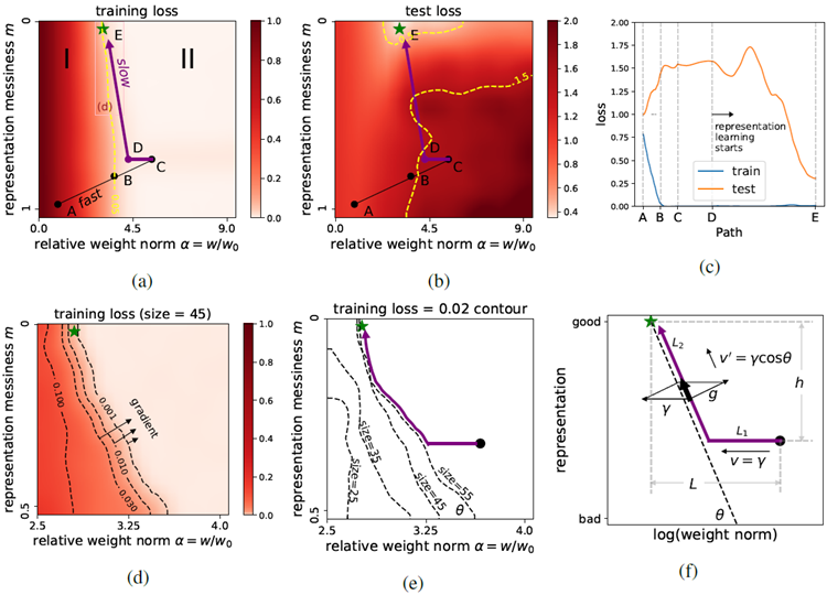
Figure 6: Loss landscapes for a toy MLP, on the 2D \((w,m)\) plane. (a) Training loss splits the plane into two regions: large loss small \(w\) (fast dynamics) and small loss large w (slow dynamics). (b) Test loss; the green star is the generalizing solution. (c) Losses along an illustrative path \(A → E\), demonstrating multiple descent; (d) zoom-in of the training loss highlighting the gradients on the boundary. (e) the boundary depends on training data size; (f) a simple illustration of grokking dynamics.
図 6: 2D \((w,m)\) 平面上のおもちゃの MLP の損失ランドスケープ。(a) トレーニング損失により、平面が 2 つの領域に分割されます。大きな損失が小さい \(w\) (高速ダイナミクス) と小さな損失が大きい w (低速ダイナミクス)。(b) テスト損失。緑の星は一般化ソリューションです。(c) 多重降下法を示す、例示的なパス \(A → E\) に沿った損失。(d) 境界上の勾配を強調表示するトレーニング損失のズームイン。(e) 境界はトレーニング データのサイズによって異なります。(f) グロッキング ダイナミクスの簡単な説明。
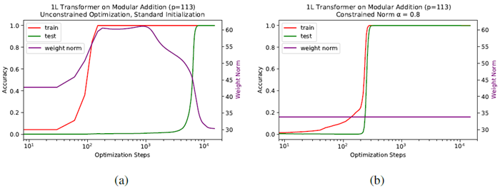
Figure 7: Training 1L transformer on modular addition (\(p = 113\)). (a) Weight norm, train accuracy, and test accuracy over time, initialized and trained normally. Weight norm first increases, and is highest during the period of overfitting, but then drops to become lower than initial weight norm when the model generalizes. (b) Constrained optimization at constant weight norm (\(α = 0.8\)) largely eliminates grokking, with test and train accuracy improving concurrently.
図7: 1Lトランスフォーマーをモジュラー加算で学習させる様子 (p = 113)。(a) 重みノルム、学習精度、テスト精度の経時変化。初期化および通常学習。重みノルムは最初は増加し、過学習期間中に最高値となるが、その後モデルが一般化すると初期の重みノルムよりも低くなる。(b) 重みノルム一定 (α = 0.8) での制約付き最適化により、グロッキングが大幅に解消され、テスト精度と学習精度が同時に向上する。
The above picture is supported by a transformer experiment: Figure 7a, shows how model norm changes over time and we see that there is an initial increase in weight norm, which peaks during overfitting, but then drops during the period of generalization to be lower than the initialization norm. For this experiment, we used the setup of (Nanda et al., 2023), training a 1-layer transformer on modular addition (\(p = 113\)). The model width \(d_{model} = 128\), with 4 attention heads, and \(d_{mlp} = 512\) with ReLU activations. We train with AdamW with a learning rate of 0.001 and weight decay \(γ= 1\).
上記の図は、Transformer実験によって裏付けられています。図7aは、モデルノルムが時間とともにどのように変化するかを示しており、重みノルムが最初に増加し、過学習中にピークに達しますが、その後、一般化期間中に低下して初期化ノルムよりも低くなります。この実験では、(Nanda et al., 2023)のセットアップを使用し、1層のTransformerをモジュラー加算(\(p = 113\))でトレーニングしました。モデル幅\(d_{model} = 128\)、アテンションヘッド4個、ReLUアクティベーション\(d_{mlp} = 512\)です。学習率0.001、重み減衰\(γ= 1\)でAdamWを使用してトレーニングしました。
Dependence of grokking on training data size Another important observation in (Power et al., 2022) is that grokking happens faster for larger training size. Our landscape analysis can also explain the data size dependence. In Figure 6e, we show the contours (training loss = 0.02) for different training sizes (25, 35, 45, 55). The contours of training size 45 and 55 both connect to the green star, meaning that generalization will eventually happen. However, the slopes of the contours are different,
i.e.,\(θ_{55} \lt θ_{45}\). Since \(t = (L + h\tanθ)/(η_Dγ)\) increases as increases, we have \(t_{55} \lt t_{45}\), i.e, more
training data leads to faster grokking. For training size 35 and 25, the contours do not connect to the green star, so generalization will not happen, no matter how long the training will be run.
グロッキングのトレーニングデータサイズへの依存性 (Power et al., 2022)におけるもう1つの重要な観察結果は、トレーニングサイズが大きいほどグロッキングが速く起こるというものです。ランドスケープ分析は、データサイズへの依存性も説明できます。図6eは、異なるトレーニングサイズ(25、35、45、55)の等高線(トレーニング損失 = 0.02)を示しています。トレーニングサイズ45と55の等高線はどちらも緑の星に接続しており、最終的には一般化が起こることを意味します。ただし、等高線の傾きは異なります。
つまり、\(θ_{55} \lt θ_{45}\)です。\(t = (L + h\tanθ)/(η_Dγ)\)は増加するにつれて増加するため、\(t_{55} \lt t_{45}\)となり、トレーニングデータが多いほどグロッキングが速くなります。トレーニング サイズ 35 および 25 の場合、輪郭は緑の星に接続されないので、トレーニングをどれだけ長く実行しても一般化は行われません。
De-grokking by constraining weight norm Guided by our understanding of grokking from the LU mechanism, we find that we can control grokking in the setting where it was first observed by Power et al. (2022) – transformers trained on algorithmic tasks. As shown in Figure 7b, reducing the initialization scale and constraining optimization to hold model weight norm constant over training brings train accuracy and test accuracy learning curves together, almost eliminating grokking.
重みノルムの制約によるグロッキングの解消 LUメカニズムから得られたグロッキングに関する理解に基づき、Powerら (2022) が最初に観察した設定、つまりアルゴリズムタスクで訓練された変換モデルにおいて、グロッキングを制御できることが分かりました。図7bに示すように、初期化スケールを縮小し、モデルの重みノルムを訓練中に一定に保つように最適化を制約することで、訓練精度とテスト精度の学習曲線が一致し、グロッキングがほぼ排除されます。
5.2 MNIST
We now study how training and test losses depend on representation messiness in the MNIST dataset.
We denote the \(28×28\) images as the raw representation \(\mathbf{R}_{raw}\). We construct a linearly separable representation \(\mathbf{R}_{linear}\) by assigning input representations proportional to their label \(y_i\), for example,
an image of a 2 is represented by a matrix with all elements being 2. Similar to Eq. (4), we use \(m \in [0,1]\) to interpolate between \(\mathbf{R}_raw\) and \(\mathbf{R}_{linear}\):
MNISTデータセットにおける表現の乱雑さが、訓練とテストの損失にどのように依存するかを考察する。
\(28×28\)枚の画像を生の表現\(\mathbf{R}_{raw}\)と表記する。ラベル\(y_i\)に比例した入力表現を割り当てることで、線形分離可能な表現\(\mathbf{R}_{linear}\)を構築する。例えば、2の画像は、すべての要素が2である行列で表現される。式(4)と同様に、\(m \in [0,1]\)を用いて\(\mathbf{R}_raw\)と\(\mathbf{R}_{linear}\)の間を補間する。
\[
\mathbf{R} = m\mathbf{R}_{raw} + (1 - m)\mathbf{R}_{linear} \tag{7}
\]
Similarly to Eq. (5), we define and plot \(\tilde{l}_{train}(w,m)\) and \(\tilde{l}_{test}(w,m)\) in Figure 8, using the full dataset N = 60000. Comparing Figures 8a and 8b reveals two things: (1) The training and test losses behave similarly; (2) Both training and test losses depend very weakly on m. This implies that the raw image representation is already quite close to being optimal, so decent test accuracy can be obtained even without learning optimal representations. As a result, grokking does not occur (Figure 8c).
式(5)と同様に、図8ではN = 60000のデータセット全体を使用して、\(\tilde{l}_{train}(w,m)\)と\(\tilde{l}_{test}(w,m)\)を定義してプロットしています。図8aと8bを比較すると、次の2つのことがわかります。(1)トレーニング損失とテスト損失は同様に振る舞います。(2)トレーニング損失とテスト損失はどちらもmに非常に弱く依存します。これは、生の画像表現が既に最適に非常に近いことを意味し、最適な表現を学習しなくても十分なテスト精度が得られます。その結果、グロッキングは発生しません(図8c)。
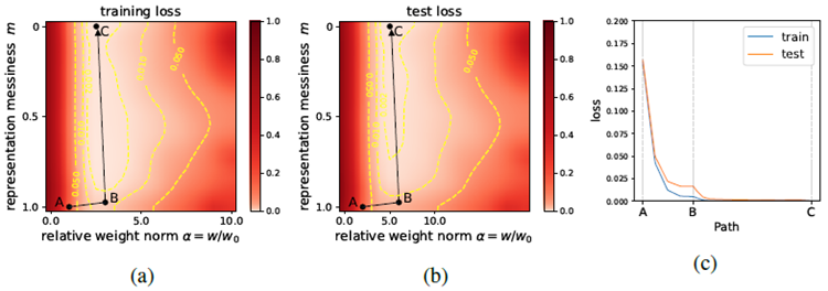
Figure 8: MNIST landscapes as functions of representation messiness \(m\) and weight norm \(w\): (a) training loss, and (b) test loss. Training and test losses do not have significant mismatch, and neither of them depend on representation strongly, which is in stark contrast to algorithmic datasets (Figure 6). (c) an illustrative path A → B → C does not manifest grokking.
図8: MNISTランドスケープを表現の乱雑さ \(m\) と重みノルム \(w\) の関数として表したもの: (a) トレーニング損失、(b) テスト損失。トレーニング損失とテスト損失には大きな不一致はなく、どちらも表現に大きく依存していない。これはアルゴリズムデータセット (図6) とは対照的である。(c) 例示的なパス A → B → C はグロッキングを示さない。
Comparing Figure 6 and 8, we see that the (strong) dependence of test performance on the representa-tion is the key to grokking: the dependence on representation is strong for algorithmic datasets, so grokking happens. By contrast, the dependence is weak for MNIST, so grokking does not happen.
図6と図8を比較すると、テストパフォーマンスの表現への(強い)依存性がグロッキングの鍵であることがわかります。アルゴリズムデータセットでは表現への依存性が強いため、グロッキングが発生します。対照的に、MNISTでは依存性が弱いため、グロッキングは発生しません。
Discussion: grokking on language models? We conjecture that grokking is more easily observed in tasks where generalization relies heavily on learning good representations (from scratch). This seems to imply the possibility of grokking on language tasks where word embeddings are key to generalization. However, we have not yet observed clear grokking signals for large language models, perhaps because: (i) the structure of languages is complicated, so the "optimal representation" for language might be much "messier" than algorithmic representations. (ii) Pre-training avoids learning representations from scratch, hence helps reduce possible grokking.
議論:言語モデルにおけるグロッキング? 一般化が(最初から)適切な表現を学習することに大きく依存するタスクでは、グロッキングがより容易に観察されると推測されます。これは、単語埋め込みが一般化の鍵となる言語タスクにおいて、グロッキングの可能性を示唆しているようです。しかし、大規模な言語モデルでは明確なグロッキングのシグナルはまだ観察されていません。その理由としては、(i)言語の構造が複雑なため、言語の「最適な表現」はアルゴリズムによる表現よりもはるかに「複雑」である可能性がある。(ii)事前学習によって表現を最初から学習する必要がなくなり、グロッキングの可能性を低減できる。
6 RELATION TO RELATED WORKS 関連研究との関係
Grokking was first observed for algorithmic datasets by (Power et al., 2022). Several formal or informal attempts have been made to understand grokking: (a) (Liu et al., 2022) attributes grokking to the slow formation of good representations. (b) (Shah, 2021) suggests that generalizable solutions achieve lower loss than overfitting solutions, providing a training signal encouraging generalization. (c) (Nanda et al., 2023) suggests grokking is a phase change due to limited data and regularization. (d) (Barak et al., 2022) suggests that generalization is due not to random search, but to hidden progress of SGD to gradually amplify a Fourier gap. (e) (Thilak et al., 2022) links grokking to the "Slingshot mechanism" specific to adaptive optimizers. (f) (Millidge, 2022) describes training as a random walk over parameters. Our conclusion supports (a)(b)(c)(d), but does not necessarily negate (e)(f).
グロッキングは、アルゴリズムデータセットにおいて、(Power et al., 2022) によって初めて観察されました。グロッキングを理解するための公式的または非公式な試みがいくつか行われてきました。(a) (Liu et al., 2022) は、グロッキングの原因を、良好な表現がゆっくりと形成されることとしています。(b) (Shah, 2021) は、一般化可能な解は過学習解よりも損失が少なく、一般化を促す学習シグナルを提供すると示唆しています。(c) (Nanda et al., 2023) は、グロッキングは限られたデータと正則化による位相変化であると示唆しています。(d) (Barak et al., 2022) は、一般化はランダム探索ではなく、SGD の隠れた進行によってフーリエギャップが徐々に増幅されることによるものだと示唆しています。(e) (Thilak et al., 2022) は、グロッキングを適応型最適化装置に特有の「スリングショットメカニズム」と関連付けています。 (f) (Millidge, 2022) は、訓練をパラメータ上のランダムウォークとして説明しています。私たちの結論は (a)(b)(c)(d) を支持するものですが、必ずしも (e)(f) を否定するものではありません。
Double descent is the phenomenon that performance first gets worse and then gets better as we increase the model size, data size, training epochs or regularization (Nakkiran et al., 2021; Yilmaz and Heckel, 2022). The typical "U" shape of test loss in this paper does not conflict with double descent, because we are plotting the weight norm instead of the number of model parameters (Ng and Ma, 2022). However, the "U"-shape should better be considered as empirically common rather than provably universal. In fact, the interaction between properties of data and inductive biases of learning algorithms can be more complicated than double descent (Chen et al., 2021; d’Ascoli et al., 2020).
二重降下法とは、モデルサイズ、データサイズ、トレーニングエポック、または正則化を増やすにつれて、パフォーマンスが最初は低下し、その後向上する現象です (Nakkiran et al., 2021; Yilmaz and Heckel, 2022)。本論文におけるテスト損失の典型的な「U」字型は、モデルパラメータの数ではなく重みノルムをプロットしているため、二重降下法とは矛盾しません (Ng and Ma, 2022)。しかし、「U」字型は、証明可能な普遍性というよりも、経験的に一般的なものと見なすべきです。実際、データの特性と学習アルゴリズムの帰納的バイアスとの相互作用は、二重降下法よりも複雑になる可能性があります (Chen et al., 2021; d’Ascoli et al., 2020)。
Initialization From the optimization perspective, initializations are usually based on the "edge of chaos" idea such that variance of features and gradients should be preserved in the forward and backward pass (Glorot and Bengio, 2010; He et al., 2015; Bahri et al., 2020; Yang and Schoenholz, 2017; Jing et al., 2017), or based on analyzing Jacobians and/or Hessians (Skorski et al., 2020). From the generalization perspective, it was shown that large initializations overfit data easily but result in poor generalization (Xu et al., 2019; Zhang et al., 2020), which agrees with our LU mechanism.
初期化 最適化の観点から見ると、初期化は通常、「カオスの端」の考え方に基づいており、特徴量と勾配の分散は順方向パスと逆方向パスで保存されるべきです(Glorot and Bengio, 2010; He et al., 2015; Bahri et al., 2020; Yang and Schoenholz, 2017; Jing et al., 2017)、またはヤコビアンやヘッセ行列の解析に基づいています(Skorski et al., 2020)。一般化の観点から見ると、大規模な初期化はデータに簡単に過剰適合しますが、一般化は不十分になることが示されています(Xu et al., 2019; Zhang et al., 2020)。これは、LUメカニズムと一致しています。
Weight decay regularization is a standard trick in machine learning and has various effects on optimization and generalization (Zhang et al., 2018; Van Laarhoven, 2017). In particular, (Lewkowycz and Gur-Ari, 2020) observes that it takes \(t \propto 1/λ\) training steps to reach maximum test performance. This is strikingly similar to the grokking time \(t \propto 1/λ\) we derived from the LU mechanism.
重み減衰正則化は機械学習における標準的な手法であり、最適化と汎化に様々な効果をもたらします (Zhang et al., 2018; Van Laarhoven, 2017)。特に、(Lewkowycz and Gur-Ari, 2020) は、最大のテスト性能に達するまでに \(t \propto 1/λ\) の訓練ステップが必要であることを指摘しています。これは、LUメカニズムから導出したグロッキング時間 \(t \propto 1/λ\) と驚くほど類似しています。
7 CONCLUSIONS 結論
This study elucidates the grokking phenomenon from the perspective of loss landscapes. Our conclusions are: (i) grokking originates from the mismatch between training and test losses ("LU" mechanism). (ii) grokking can happen in various models for a wide range of datasets, although the grokking signature is usually most dramatic for algorithmic datasets. (iii) The dramaticness of grokking depends on how much the task relies on learning representations. This work not only reveals the mechanism of grokking, but also shows that reduced landscape analysis is a useful tool for characterizing data-model interaction and representation learning.
本研究は、グロッキング現象を損失ランドスケープの観点から解明する。結論は以下の通りである。(i) グロッキングは、訓練用損失とテスト用損失の不一致(「LU」メカニズム)に起因する。(ii) グロッキングは様々なモデルで、幅広いデータセットにおいて発生する可能性があるが、グロッキングの顕著な特徴は通常、アルゴリズムデータセットで最も顕著である。(iii) グロッキングの顕著さは、タスクが表現学習にどの程度依存しているかによって決まる。本研究は、グロッキングのメカニズムを明らかにするだけでなく、縮退ランドスケープ解析がデータとモデルの相互作用および表現学習を特徴付けるための有用なツールであることを示している。
ACKNOWLEDGEMENT 謝辞
We thank Wenxian Shi, Niklas Nolte, Ouail Kitouni and Mike Williams for helpful discussions. This work was supported by The Casey and Family Foundation, the Foundational Questions Institute, the Rothberg Family Fund for Cognitive Science, the NSF Graduate Research Fellowship (Grant No. 2141064), and the NSF AI Institute for Artificial Intelligence and Fundamental Interactions (IAIFI) through NSF Grant No. PHY-2019786.
有益な議論をしてくださったWenxian Shi氏、Niklas Nolte氏、Ouail Kitouni氏、Mike Williams氏に感謝します。本研究は、Casey and Family Foundation、Foundational Questions Institute、Rothberg Family Fund for Cognitive Science、NSF Graduate Research Fellowship(助成金番号2141064)、およびNSF AI Institute for Artificial Intelligence and Fundamental Interactions(IAIFI)(NSF助成金番号PHY-2019786)の支援を受けています。
REFERENCES 参考文献
-
Alethea Power, Yuri Burda, Harri Edwards, Igor Babuschkin, and Vedant Misra. Grokking: Gen-eralization beyond overfitting on small algorithmic datasets. arXiv preprint arXiv:2201.02177, 2022.
-
Ziming Liu, Ouail Kitouni, Niklas Nolte, Eric J Michaud, Max Tegmark, and Mike Williams. Towards understanding grokking: An effective theory of representation learning. arXiv preprint arXiv:2205.10343, 2022.
-
Vimal Thilak, Etai Littwin, Shuangfei Zhai, Omid Saremi, Roni Paiss, and Joshua Susskind. The slingshot mechanism: An empirical study of adaptive optimizers and the grokking phenomenon. arXiv preprint arXiv:2206.04817, 2022.
-
Boaz Barak, Benjamin L Edelman, Surbhi Goel, Sham Kakade, Eran Malach, and Cyril Zhang. Hidden progress in deep learning: Sgd learns parities near the computational limit. arXiv preprint arXiv:2207.08799, 2022.
-
Stanislav Fort and Adam Scherlis. The goldilocks zone: Towards better understanding of neural network loss landscapes. In Proceedings of the AAAI Conference on Artificial Intelligence, volume 33, pages 3574–3581, 2019.
-
Preetum Nakkiran, Gal Kaplun, Yamini Bansal, Tristan Yang, Boaz Barak, and Ilya Sutskever. Deep double descent: Where bigger models and more data hurt. Journal of Statistical Mechanics: Theory and Experiment, 2021(12):124003, 2021.
-
Andrew Ng and Tengyu Ma. Cs229 lecture notes. https://cs229.stanford.edu/lectures-spring2022/main_notes.pdf, page 115, 2022.
-
Samuel S Schoenholz, Justin Gilmer, Surya Ganguli, and Jascha Sohl-Dickstein. Deep information propagation. arXiv preprint arXiv:1611.01232, 2016.
-
Ge Yang and Samuel Schoenholz. Mean field residual networks: On the edge of chaos. Advances in neural information processing systems, 30, 2017.
-
Li Deng. The mnist database of handwritten digit images for machine learning research. IEEE Signal Processing Magazine, 29(6):141–142, 2012.
-
Sepp Hochreiter and Jürgen Schmidhuber. Long short-term memory. Neural computation, 9(8): 1735–1780, 1997.
-
Andrew L. Maas, Raymond E. Daly, Peter T. Pham, Dan Huang, Andrew Y. Ng, and Christopher Potts. Learning word vectors for sentiment analysis. In Proceedings of the 49th Annual Meeting of the Association for Computational Linguistics: Human Language Technologies, pages 142–150, Portland, Oregon, USA, June 2011. Association for Computational Linguistics. URL http: //www.aclweb.org/anthology/P11-1015.
-
Raghunathan Ramakrishnan, Pavlo O Dral, Matthias Rupp, and O Anatole von Lilienfeld. Quantum chemistry structures and properties of 134 kilo molecules. Scientific Data, 1, 2014.
-
Neel Nanda, Lawrence Chan, Tom Liberum, Jess Smith, and Jacob Steinhardt. Progress measures for grokking via mechanistic interpretability. arXiv preprint arXiv:2301.05217, 2023.
-
Rohin Shah. Alignment Newsletter #159. https:// www.alignmentforum.org/posts/zvWqPmQasssaAWkrj/
an-159-building-agents-that-know-how-to-experiment-by#DEEP_ LEARNING_, 2021.
-
Beren Millidge. Grokking ’grokking’. https://beren.io/ 2022-01-11-Grokking-Grokking/, 2022.
-
Fatih Furkan Yilmaz and Reinhard Heckel. Regularization-wise double descent: Why it occurs and how to eliminate it. In 2022 IEEE International Symposium on Information Theory (ISIT), pages 426–431. IEEE, 2022.
-
Lin Chen, Yifei Min, Mikhail Belkin, and Amin Karbasi. Multiple descent: Design your own generalization curve. Advances in Neural Information Processing Systems, 34:8898–8912, 2021.
-
Stéphane d’Ascoli, Levent Sagun, and Giulio Biroli. Triple descent and the two kinds of overfitting: Where & why do they appear? Advances in Neural Information Processing Systems, 33:3058–3069, 2020.
-
Xavier Glorot and Yoshua Bengio. Understanding the difficulty of training deep feedforward neural networks. In Proceedings of the thirteenth international conference on artificial intelligence and statistics, pages 249–256. JMLR Workshop and Conference Proceedings, 2010.
-
Kaiming He, Xiangyu Zhang, Shaoqing Ren, and Jian Sun. Delving deep into rectifiers: Surpassing human-level performance on imagenet classification. In Proceedings of the IEEE international conference on computer vision, pages 1026–1034, 2015.
-
Yasaman Bahri, Jonathan Kadmon, Jeffrey Pennington, Sam S Schoenholz, Jascha Sohl-Dickstein, and Surya Ganguli. Statistical mechanics of deep learning. Annual Review of Condensed Matter Physics, 11(1), 2020.
-
Li Jing, Yichen Shen, Tena Dubcek, John Peurifoy, Scott Skirlo, Yann LeCun, Max Tegmark, and Marin Soljacic. Tunable efficient unitary neural networks (eunn) and their application to rnns. In International Conference on Machine Learning, pages 1733–1741. PMLR, 2017.
-
Maciej Skorski, Alessandro Temperoni, and Martin Theobald. Revisiting initialization of neural networks. arXiv preprint arXiv:2004.09506, 2020.
-
Zhi-Qin John Xu, Yaoyu Zhang, and Yanyang Xiao. Training behavior of deep neural network in frequency domain. In International Conference on Neural Information Processing, pages 264–274. Springer, 2019.
-
Yaoyu Zhang, Zhi-Qin John Xu, Tao Luo, and Zheng Ma. A type of generalization error induced by initialization in deep neural networks. In Mathematical and Scientific Machine Learning, pages 144–164. PMLR, 2020.
-
Guodong Zhang, Chaoqi Wang, Bowen Xu, and Roger Grosse. Three mechanisms of weight decay regularization. arXiv preprint arXiv:1810.12281, 2018.
-
Twan Van Laarhoven. L2 regularization versus batch and weight normalization. arXiv preprint arXiv:1706.05350, 2017.
-
Aitor Lewkowycz and Guy Gur-Ari. On the training dynamics of deep networks with l_2 regulariza-tion. Advances in Neural Information Processing Systems, 33:4790–4799, 2020.
-
Diederik P Kingma and Jimmy Ba. Adam: A method for stochastic optimization. arXiv preprint arXiv:1412.6980, 2014.
Appendix 付録
A EXPERIMENT DETAILS 実験の詳細
Sentiment analysis of text IMDb (Maas et al., 2011) includes 50k movie reviews to be classified as being positive or negative. To pre-process the data, we extract the 1000 most frequent words and tokenize each review into an array of token indices. Less frequent words are ignored, and each review array is padded to length 500. We adopt the LSTM model (Hochreiter and Schmidhuber, 1997) to perform the classification, with two layers, embedding dimension 64, and hidden dimension 128. We use the Adam optimizer (Kingma and Ba, 2014) with learning rate 0.001 to minimize the binary cross entropy loss. We hold back 25% of the dataset for testing.
テキストの感情分析 IMDb (Maas et al., 2011) には、肯定的か否定的かに分類される 5 万件の映画レビューが含まれています。データを前処理するために、最も頻繁に使用される 1000 語を抽出し、各レビューをトークン インデックスの配列にトークン化します。頻度の低い語は無視され、各レビュー配列は長さ 500 にパディングされます。分類には LSTM モデル (Hochreiter and Schmidhuber, 1997) を採用し、2 つのレイヤー、埋め込み次元 64、非表示次元 128 を使用します。バイナリ クロス エントロピー損失を最小限に抑えるため、学習率 0.001 で Adam オプティマイザー (Kingma and Ba, 2014) を使用します。データセットの 25% をテスト用に残しておきます。
Molecules QM9 is a database for small molecules and their properties. We use a graph convolutional neural network (GCNN) to predict the isotropic polarizability. The GCNN contains 2 convolutional layers with ReLU activation, followed by a linear layer. We use the Adam optimizer with learning rate 0.001 to minimize the MSE loss. We split the dataset into 50/50 train/test.
分子 QM9は、小分子とその特性に関するデータベースです。グラフ畳み込みニューラルネットワーク(GCNN)を用いて等方分極率を予測します。GCNNは、ReLU活性化を用いた2つの畳み込み層と、それに続く線形層で構成されています。MSE損失を最小化するため、学習率0.001のAdamオプティマイザーを使用しています。データセットは学習用とテスト用に50/50に分割しています。
MNIST We train width-200 depth-3 ReLU MLPs on the MNIST dataset with MSE loss. We use the AdamW optimizer with a learning rate of 0.001 and a batch size of 200.
MNIST MNISTデータセットを用いて、幅200、深さ3のReLU MLPをMSE損失付きで学習します。AdamWオプティマイザーを使用し、学習率0.001、バッチサイズ200で学習します。
B REDUCED LOSS FOR MODULAR ADDITION WITH TRANSFORMERS トランスフォーマーによるモジュール追加で損失を低減
In Figure 9 we show reduced loss landscape plots for transformers trained on modular addition. We use the setup of Nanda et al. (2023) and train a 1-layer transformer on modular addition (\(p = 113\)) with \(d_{model} = 128\), 4 attention heads, and \(d_{mlp} = 512\) with ReLU activations. We train with a learning
rate of 0.001 while constraining model weight norm, for a variety of and a variety of train set fractions. The LU shape holds for \(α \in [0,1,4]\) (some optimization issue may be responsible for the rise in train loss for \(α> 4\)). We see the critical train set size is approximately 0.25, in line with earlier studies on grokking.
図9に、モジュラー加算でトレーニングされたTransformerの損失削減ランドスケーププロットを示します。Nanda et al. (2023)のセットアップを使用し、1層のTransformerを、\(d_{model} = 128\)、4つのアテンションヘッド、および\(d_{mlp} = 512\)でReLUアクティベーションを使用して、モジュラー加算でトレーニングします(\(p = 113\))。モデルの重みノルムを制約しながら、学習率0.001で、さまざまなトレーニングセットの割合でトレーニングします。LUの形状は\(α \in [0,1,4]\)に当てはまります(\(α> 4\)でのトレーニング損失の上昇は、何らかの最適化の問題が原因である可能性があります)。臨界トレーニングセットサイズは約0.25であり、これはgrokkingに関する以前の研究と一致しています。
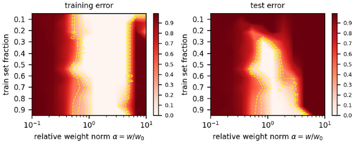
Figure 9: Reduced loss landscapes for transformers trained on modular addition, the original setting where grokking was observed.
図 9: グロッキングが観察された元の設定である、モジュール追加でトレーニングされたトランスフォーマーの損失ランドスケープの削減。
C TIME TO GENERALIZE VERSUS WEIGHT DECAY 一般化の時間と重み減衰
In our discussion of the “LU mechanism” as an explanation for grokking in Section 2, we predicted
that the training time required for a model to generalize should be \(t \propto γ^{-1}\) where \(γ\) is the weight decay. To test this, we perform a grid search over weight decays \(γ\) and plot the number of training steps required for models to reach a specified level of test accuracy in Figure 10a-10b. We also show full training curves for these runs in Figure 10c-10d. We perform experiments in two setups:
第2節でグロッキングを説明する「LUメカニズム」について議論した際、モデルが汎化するために必要な訓練時間は \(t \propto γ^{-1}\) であると予測しました。ここで \(γ\) は重みの減衰です。これを検証するために、重みの減衰 \(γ\) に対してグリッドサーチを実行し、モデルが特定のテスト精度レベルに達するために必要な訓練ステップ数を図10a-10bにプロットしました。また、これらの実行における完全な訓練曲線を図10c-10dに示します。実験は2つの設定で行いました。
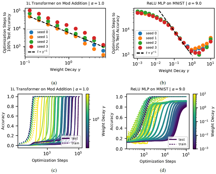
Figure 10: Time to generalize as a function of weight decay: we investigate to what extent the relation
\(t \propto γ^{-1}\) holds, where \(t\) is number of training steps needed for the model to generalize and \(γ\) is the AdamW weight decay. When a lower weight decay is used, models spend longer in the period of overfitting before eventually generalizing. We show the generalization time t as a function of in (a)-(b) and full training curves for these runs in (c)-(d).
図10: 重み減衰の関数としての汎化時間:関係式
\(t \propto γ^{-1}\) がどの程度成立するかを調べる。ここで、\(t\) はモデルが汎化するために必要なトレーニングステップ数、\(γ\) は AdamW の重み減衰である。より低い重み減衰が使用される場合、モデルは最終的に汎化されるまでの過学習期間が長くなる。(a)-(b) に汎化時間 t を関数として示し、(c)-(d) にこれらの実行における完全なトレーニング曲線を示す。
-
(a) Transformer on modular addition: We use the replication of grokking from Nanda et al. (2023) and train a 1-layer transformer on modular addition (\(p = 113\) and a train set fraction of 0.3) where \(d_{model} = 128\), with 4 attention heads, \(d_{mlp} = 512\), ReLU activations, and an AdamW learning rate of 0.001. From Figure 10a, we find that \(t \propto γ^{-1}\) holds across roughly two orders of magnitude of \(t\) and \(γ\). There is some seed dependence on the generalization
time (some seeds consistently require longer to generalize), but for each seed (corresponding
to a particular model initialization) the relation \(t \propto γ^{-1}\) appears to fit the data well.
(a) モジュラー加算に関するトランスフォーマー: Nandaらによるgrokkingの複製を使用します。 (2023) を用いて、モジュラー加算(p = 113\)、訓練セットの割合 0.3)で 1層トランスフォーマーを訓練します。ここで、\(d_{model} = 128\)、アテンション ヘッド 4 つ、\(d_{mlp} = 512\)、ReLU アクティベーション、AdamW 学習率 0.001 です。図 10a から、\(t\) と \(γ\) がおよそ 2 桁にわたって \(t\) と \(γ\) にわたって成立していることがわかります。一般化時間にはシードに多少の依存性があります(シードによっては、一般化に一貫して長い時間がかかります)が、各シード(特定のモデル初期化に対応)について、関係 \(t \propto γ^{-1}\) がデータによく適合しているように見えます。
-
(b) ReLU MLP on MNIST: We train ReLU MLPs on MNIST as described in Appendix A. We use an \(α= 9.0\) and train on a reduced training set of 1000 samples to delay generalization /
induce grokking. From Figure 10b, we find that for \(γ\) roughly between 0.1 and 1.0 the relation
\(t \propto γ^{-1}\) holds. Very high values of weight decay seem to mess with optimization. On the other hand, with very low weight decay the model generalizes faster than naively expected, perhaps due to implicit regularization.
(b) MNIST 上の ReLU MLP:付録 A で説明したように、MNIST 上で ReLU MLP を学習します。\(α = 9.0\) を使用し、汎化を遅らせ、グロッキングを促します。図 10b から、\(γ\) がおよそ 0.1 から 1.0 の間であれば、関係式
\(t \propto γ^{-1}\) が成り立つことがわかります。重みの減衰が非常に高いと、最適化がうまくいかないようです。一方、重みの減衰が非常に低いと、モデルは単純に予想されるよりも速く汎化します。これはおそらく暗黙的な正則化によるものと考えられます。
D SECTION 5.1 SETUP 5.1節の設定
Architecture Similar to Liu et al. (2022), the decoder architecture is an MLP with hard coded addition. Each input symbol \(i\) is encoded to a scalar \(E_i\). Each output symbol \(k\) is represented by a 30D random vector \(\hat{\mathbf{Y}}_k\). We consider addition with base \(p\), so input \(0 \leq i, j \leq p-1\) and output \(0 \leq k = i + j \leq 2(p-1)\). We denote representation as \(\mathbf{R} = \{E_0,E_1,\cdots,E_{p-1}\}\). The MLP has
two hidden layers, with neurons 1-200-200-30 in each layer and ReLU activations. Given a training sample \((E_i,E_j)→\mathbf{Y}_k\) where \(i + j = k\), the prediction of the MLP decoder is
アーキテクチャ Liu et al. (2022) と同様に、デコーダのアーキテクチャはハードコードされた加算を備えたMLPです。各入力シンボル \(i\) はスカラー \(E_i\) にエンコードされます。各出力シンボル \(k\) は30次元ランダムベクトル \(\hat{\mathbf{Y}}_k\) で表されます。基数 \(p\) の加算を考えると、入力 \(0 \leq i, j \leq p-1\)、出力 \(0 \leq k = i + j \leq 2(p-1)\) となります。表現を \(\mathbf{R} = \{E_0,E_1,\cdots,E_{p-1}\}\) と表記します。MLPには2つの隠れ層があり、各層にはニューロン1-200-200-30とReLU活性化があります。訓練サンプル\((E_i,E_j)→\mathbf{Y}_k\) (\(i + j = k\)) が与えられた場合、MLPデコーダーの予測は次のようになる。
\[
\mathbf{Y}_k = Dec_w(E_i + E_j) \tag{8}
\]
and the loss function being the mean squared error (MSE) between \(\mathbf{Y}_k\) and \(\hat{\mathbf{Y}}_k\), and \(\mathbf{w}\) being the decoder weight. Although the common setup of grokking is to make both the representation \(\mathbf{R}\) and the decoder \(\mathbf{w}\) trainable, we will freeze part of them for easier analysis. This is where it could be a bit confusing, so we explicitly distinguish three setups: landscape analysis, reduced trajectory analysis and full trajectory analysis. Each setup have different subset of trainable parameters, as shown in Table 1.
損失関数は\(\mathbf{Y}_k\)と\(\hat{\mathbf{Y}}_k\)の平均二乗誤差(MSE)、\(\mathbf{w}\)はデコーダーの重みです。グロッキングの一般的な設定では、表現\(\mathbf{R}\)とデコーダー\(\mathbf{w}\)の両方を学習可能にしますが、ここでは分析を容易にするためにその一部を固定します。ここが少し分かりにくい点であるため、ランドスケープ解析、縮小軌道解析、完全軌道解析の3つの設定を明確に区別します。表1に示すように、各設定には学習可能なパラメーターの異なるサブセットがあります。
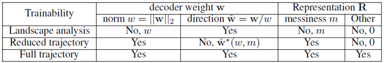
Table 1: Threes setups used in this paper, with different set of parameters trainable.
表 1: この論文で使用した 3 つのセットアップ (トレーニング可能なさまざまなパラメータ セット)。
Landscape analysis Both the representation \(\mathbf{R}\) and weight norm \(w\) are fixed. Only the weight direction \(\hat{\mathbf{w}}\) is trainable. The representation \(\mathbf{R}\) is fixed according to Eq. (4), which is dependent on \(m\), the representation messiness. The decoder has fixed weight norm w, but the weight direction w is trainable. For each fixed \((w,m)\), we minimize training loss over \(\hat{\mathbf{w}}\) to get
ランドスケープ分析 表現\(\mathbf{R}\)と重みノルム\(w\)はともに固定である。重み方向\(\hat{\mathbf{w}}\)のみが学習可能である。表現\(\mathbf{R}\)は式(4)に従って固定され、これは表現の複雑さ \(m\) に依存する。デコーダーは重みノルムwを固定しているが、重み方向wは学習可能である。固定された各\((w,m)\)について、\(\hat{\mathbf{w}}\)の学習損失を最小化して、
\[
\hat{\mathbf{w}}^*(w,m) = \text{arg}\min\limits_{\hat{\mathbf{w}}} l_{train}(w,m,\hat{\mathbf{w}}) \tag{9}
\]
and define reduced training and test loss, as in Eq. (5). The minimization is implemented by the
Adam optimizer with learning rate 10-34 steps. Although \((w,m)\) are not trainable, we repeat the above minimization independently for different \((w,m)\). In Figure 6 (a)(b)(d), the background heatmaps belong to landscape analysis.
式(5)のように、訓練損失とテスト損失の低減を定義します。この最小化は、学習率10-3、104ステップのAdam最適化器によって実装されます。\((w,m)\)は学習できませんが、上記の最小化を異なる\((w,m)\)に対して独立に繰り返します。図6(a)(b)(d)の背景ヒートマップはランドスケープ分析に属します。
Reduced trajectory analysis is a “thought experiment" based on landscape analysis. Since full trajectory analysis can be intractable due to too high dimensions, we try to reduce the trajectory anaysis to 2D, by making two assumptions about the real dynamics: (1) Scale separation: the dynamics of \(\hat{\mathbf{w}}\) is much faster than the dynamics along \(w\) and along \(m\), such that \(\hat{\mathbf{w}}(t) = \hat{\mathbf{w}}^*(w(t),m(t))\) is valid at every moment during training. (2) Representation evolution is linear, i.e., interpolating between initial random Gaussian and final linear representation. With these two assumptions, the training dynamics is effectively reduced to 2D, depending only on \((w,m)\), obeying Eq. (6). In Figure 6 (a)(b)(c), the path \(A → E\) belongs to reduced trajectory analysis.
縮小軌道解析は、ランドスケープ解析に基づく「思考実験」です。完全な軌道解析は次元が高すぎるために扱いにくい場合があるため、実際のダイナミクスについて次の 2 つの仮定を立てて、軌道解析を 2D に縮小します。(1) スケール分離: \(\hat{\mathbf{w}}\) のダイナミクスは、\(w\) や \(m\) に沿ったダイナミクスよりもはるかに高速であるため、トレーニング中のすべての瞬間で \(\hat{\mathbf{w}}(t) = \hat{\mathbf{w}}^*(w(t),m(t))\) が有効です。(2) 表現の進化は線形です。つまり、初期のランダム ガウス表現と最終的な線形表現の間を補間します。これら2つの仮定のもと、訓練ダイナミクスは実質的に2次元に縮約され、\((w,m)\)のみに依存し、式(6)に従います。図6(a)(b)(c)において、パス\(A → E\)は縮小軌道解析に属します。
Admittedly the reduced trajectory may deviate from the full trajectory since the assumptions may not be met, but it can shed light on the full trajectory: the weight norm first increases and then increases, and the decrease of weight norm is highly correlated with generalization (please see Appendix ?? and Figure 7.
確かに、仮定が満たされない可能性があるため、縮小された軌道は完全な軌道から逸脱する可能性がありますが、完全な軌道を明らかにすることができます。重みノルムは最初に増加し、その後増加し、重みノルムの減少は一般化と高い相関関係にあります (付録 ?? および図 7 を参照してください)。
E MNIST EXPERIMENTS WITH CROSS ENTROPY LOSS 交差エントロピー損失を用いたMNIST実験
To respond to a reviewer’s concern that our use of the MSE loss is the “secret" to get grokking on MNIST (Figure 3), we reran our experiments with the cross entropy (CE) loss. The results are qualitatively similar, with some quantitative differences.
MSE損失の使用がMNIST(図3)をグロッキングする(理解する)ための「秘訣」であるという査読者の懸念に応えるため、交差エントロピー(CE)損失を用いて実験を再実行しました。結果は定性的には類似していますが、定量的には若干の違いがありました。
Landscape analysis ランドスケープ解析
Comparing Figure 3 (MSE) and Figure 11 (CE), we notice the they are qualitatively similar: (1) for small datasets, the reduced training error and test error resemble an “L" and “U" against the weight norm, respectively; (2) for large datasets, the “U" becomes more like “L", i.e., the mismatch between the reduced training and test error is small. However, a quantitative difference exist: CE produces a broader “Goldilocks zone" (the weight range where generalization happens) than MSE. This implies that to induce grokking with CE, we need to increase the weight norm to a larger value (say α = 100).
図 3 (MSE) と図 11 (CE) を比較すると、定性的に類似していることがわかります。(1) データセットが小さい場合、削減されたトレーニング エラーとテスト エラーは、重みノルムに対してそれぞれ「L」と「U」に似ています。(2) データセットが大きい場合、「U」は「L」に近くなります。つまり、削減されたトレーニング エラーとテスト エラーの不一致は小さくなります。ただし、定量的な違いもあります。CE は、MSE よりも広い「ゴルディロックス ゾーン」(一般化が発生する重みの範囲) を生成します。これは、CE によるグロッキングを誘発するには、重みノルムをより大きな値 (たとえば α = 100) に増やす必要があることを意味します。
Training dynamics トレーニングダイナミクス
We are able to observe delayed generalization during trianing on MNIST with cross entropy loss, but doing so requires a higher than was necessary when using MSE loss, as predicted by the reduced loss landscapes in Figure 11. Figure 12 shows training trajectories from a 3-layer ReLU MLP on MNIST trained with cross entropy loss with α = 100 and D = 200. We see that test accuracy rises to 30-40% early in training, then plateaus for an extended period, before increasing to 75% while train accuracy remains at 100%. While the dynamics are not as clean as with MSE loss, since test accuracy first plateaus at better-than-random accuracy, we think it is still fair to classify these dynamics as “grokking” due to the improvement in generalization late in training after a plateau.
クロス エントロピー損失のある MNIST での学習中に遅延一般化を観察できますが、そのためには、図 11 の減少した損失ランドスケープによって予測されるように、MSE 損失を使用する場合よりも高いレベルが必要です。図 12 は、α = 100、D = 200 でクロス エントロピー損失を使用して学習した MNIST 上の 3 層 ReLU MLP の学習軌跡を示しています。テスト精度は学習の初期に 30~40% まで上昇し、その後長期間にわたって横ばい状態になった後、学習精度が 100% のまま 75% まで増加することがわかります。ダイナミクスは MSE 損失の場合ほど明確ではありませんが、テスト精度は最初にランダムよりも優れた精度で横ばい状態になるため、学習後期に一般化が向上するため、これらのダイナミクスを「grokking」として分類することは依然として妥当であると考えられます。
Figure 11: MNIST with the cross entropy loss (as opposed to the MSE loss used in Figure 3). (a) reduced training error, (b) reduced test error. (c) "LU" still holds for the cross entropy loss, but the effect is milder than the MSE loss. In particular, the “Goldilocks zone" (the weight range where generalization happens) is broader.
図11:交差エントロピー損失を用いたMNIST(図3で使用したMSE損失とは対照的)。(a) 学習誤差の減少、(b) テスト誤差の減少。(c) 交差エントロピー損失でも「LU」は成立するが、その影響はMSE損失よりも小さい。特に、「ゴルディロックスゾーン」(汎化が起こる重みの範囲)が広くなっている。
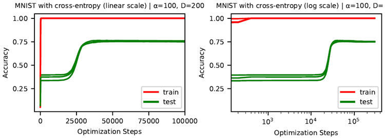
Figure 12: Training curves using cross entropy loss on MNIST. We are still able to observe delayed generalization on MNIST using cross entropy loss, though test accuracy first plateaus at higher than random-guess accuracy.
図12: MNISTにおけるクロスエントロピー損失を用いたトレーニング曲線。クロスエントロピー損失を用いたMNISTでも遅延汎化が観察されますが、テスト精度はランダム推測精度よりも高い値で一旦横ばいになります。