The receptive fields of simple cells in mammalian primary visual
cortex can be characterized as being spatially localized,
oriented1-4 and bandpass (selective to structure at different
spatial scales), comparable to the basis functions of wavelet
transforms5,6. One approach to understanding such response
properties of visual neurons has been to consider their relation-
ship to the statistical structure of natural images in terms of
efficient coding7-12. Along these lines, a number of studies have
attempted to train unsupervised learning algorithms on natural
images in the hope of developing receptive fields with similar
properties13-18, but none has succeeded in producing a full set that
spans the image space and contains all three of the above
properties. Here we investigate the proposal8,12 that a coding
strategy that maximizes sparseness is sufficient to account for
these properties. We show that a learning algorithm that
attempts to find sparse linear codes for natural scenes will
develop a complete family of localized, oriented, bandpass recep-
tive fields, similar to those found in the primary visual cortex. The
resulting sparse image code provides a more efficient representa-
tion for later stages of processing because it possesses a higher
degree of statistical independence among its outputs.
哺乳類の一次視覚皮質における単純細胞の受容野は、空間的に局在し、方向性を持ち1-4、帯域通過性(異なる空間スケールでの構造を選択的に有する)を持つことで特徴付けられ、ウェーブレット変換の基底関数5,6に匹敵します。視覚ニューロンのこのような応答特性を理解するための一つのアプローチは、効率的な符号化7-12の観点から、自然画像の統計的構造との関係を考察することです。この観点から、多くの研究において、自然画像を用いて教師なし学習アルゴリズムを訓練し、同様の特性を持つ受容野を開発しようと試みられてきました13-18。しかし、画像空間全体に広がり、上記3つの特性すべてを含む完全な受容野セットを作成することに成功した研究はありません。本稿では、スパース性を最大化する符号化戦略がこれらの特性を説明するのに十分であるという提案8,12を検証する。自然風景のスパース線形符号を見つけようとする学習アルゴリズムは、一次視覚野に見られるものと同様の、局所的かつ方向性のある帯域通過受容野の完全なファミリーを開発することを示す。結果として得られるスパース画像符号は、出力間の統計的独立性が高いため、後段の処理段階でより効率的な表現を提供する。
We start with the basic assumption that an image, \(I(x, y)\), can be
represented in terms of a linear superposition of (not necessarily
orthogonal) basis functions, \(\phi_i(x,y)\):
まず、画像 \(I(x, y)\) は、(必ずしも直交ではない)基底関数 \(\phi_i(x, y)\) の線形重ね合わせで表現できるという基本的な仮定から始めます。
\[
I(x,y) = \sum_i a_i \phi_i(x,y) \tag{1}
\]
The image code is determined by the choice of basis functions, \(\phi_i\).
The coefficients, \(a_i\), are dynamic variables that change from one
image to the next. The goal of efficient coding is to find a set of \(\phi_i\) that forms a complete code (that is, spans the image space) and
results in the coefficient values being as statistically independent
as possible over an ensemble of natural images. The reasons for
desiring statistical independence have been elaborated else-
where9,12,19, but can be summarized briefly as providing a strategy
for extracting the intrinsic structure in sensory signals.
画像コードは、基底関数 \(\phi_i\) の選択によって決定されます。
係数 \(a_i\) は、画像ごとに変化する動的な変数です。効率的な符号化の目標は、完全なコード(つまり、画像空間全体にわたる)を形成し、自然画像の集合全体にわたって可能な限り統計的に独立した係数値となるような \(\phi_i\) の集合を見つけることです。統計的独立性が求められる理由は、既に他の文献9,12,19で詳しく説明されていますが、簡単にまとめると、感覚信号の本質的な構造を抽出するための戦略を提供するということになります。
One line of approach to this problem is based on principal-
components analysis14,15,20, in which the goal is to find a set of
mutually orthogonal basis functions that capture the directions of
maximum variance in the data and for which the coefficients are
pairwise decorrelated, \(\langle a_ia_j\rangle = \langle a_i\rangle\langle a_j\rangle\). The receptive fields that
result from this process are not localized, however, and the vast
majority do not at all resemble any known cortical receptive fields
(Fig. 1). Principal components analysis is appropriate for captur-
ing the structure of data that are well described by a gaussian
cloud, or in which the linear pairwise correlations are the most
important form of statistical dependence in the data. But natural
scenes contain many higher-order forms of statistical structure,
and there is good reason to believe they form an extremely non-
gaussian distribution that is not at all well captured by orthogonal
components12. Lines and edges, especially curved and fractal-like
edges, cannot be characterized by linear pairwise statistics6,21 and
so a method is needed for evaluating the representation that can
take into account higher-order statistical dependences in the
data.
この問題へのアプローチの一つは主成分分析14,15,20に基づくものであり、その目的は、データ内の最大分散の方向を捉え、かつ係数が対ごとに相関が取れていない、互いに直交する基底関数の集合を見つけることである \(\langle a_i a_j\rangle = \langle a_i\rangle\langle a_j\rangle\)。しかし、このプロセスによって生じる受容野は局所化されておらず、その大部分は既知の皮質受容野とは全く類似していない(図1)。主成分分析は、ガウス分布でよく記述されるデータ、または線形対相関がデータにおける最も重要な統計的依存性であるデータの構造を捉えるのに適している。しかし、自然風景には多くの高次の統計構造が含まれており、それらは直交成分では全く捉えられない極めて非ガウス分布を形成すると考えられる十分な理由があります12。線やエッジ、特に曲線やフラクタル状のエッジは、線形ペアワイズ統計では特徴付けることができません6,21。そのため、データ内の高次の統計的依存性を考慮できる表現を評価する方法が必要です。
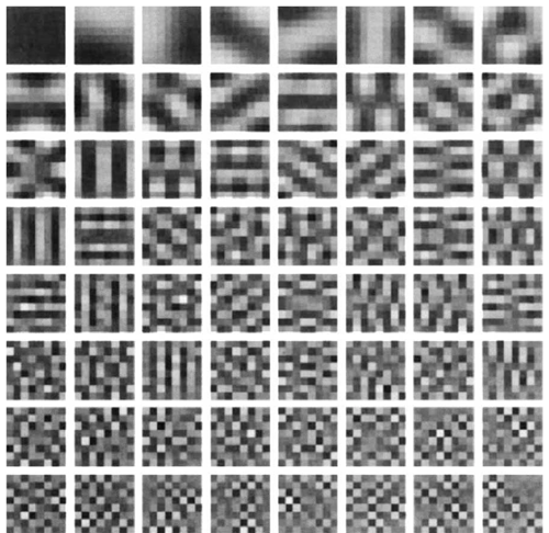
FIG. 1 Principal components calculated on 8 x 8 image patches extracted
from natural scenes by using Sanger’s rule14. The full set of 64 components
is shown, ordered by their variance (by columns, then by rows). The oriented
structure of the first few principal components does not arise as a result of
the oriented structures in natural images, but rather because these
functions are composed of a small number of low-frequency components
(the lowest spatial frequencies account for the greatest part of the variance
in natural scenes8). Reconstructions based solely on the first row of
functions will merely yield blurry images. Identical-looking components
are obtained for images with the same amplitude spectrum as natural
images but with randomized phases (that is, 1/f noise).
図1:サンガー則14を用いて自然風景から抽出した8×8の画像パッチに基づいて計算された主成分。64個の成分すべてが、分散(列、行)順に並べられて示されている。最初の数個の主成分の配向構造は、自然画像の配向構造の結果として生じたものではなく、これらの関数が少数の低周波成分で構成されているために生じたものである(自然風景における分散の大部分は、最も低い空間周波数によって説明される8)。最初の行の関数のみに基づいて再構成すると、ぼやけた画像しか得られない。自然画像と同じ振幅スペクトルを持ちながら、位相がランダム化された画像(つまり、1/fノイズ)では、同じように見える成分が得られる。
The existence of any statistical dependences among a set of
variables may be discerned whenever the joint entropy is less than
the sum of individual entropies, \(H(a_1,a_2,...,a_n) \lt \sum_i H(a_i)\), otherwise the two quantities will equal. Assuming that we have some
way of ensuring that information in the image (joint entropy) is
preserved, then a possible strategy for reducing statistical depen-
dences is to lower the individual entropies, \(H(a_i)\), as much as
possible. In Barlow’s terms19, we seek a minimum-entropy code.
We conjecture that natural images have ‘sparse structure’— that
is, any given image can be represented in terms of a small number
of descriptors out of a large set8,12 — and so we shall seek a specific
form of low-entropy code in which the probability distribution of
each coefficient’s activity is unimodal and peaked around zero.
変数集合間の統計的依存関係の存在は、結合エントロピーが個々のエントロピーの合計\(H(a_1,a_2,...,a_n) \lt \sum_i H(a_i)\)よりも小さい場合に判断できます。そうでない場合、2つの量は等しくなります。画像内の情報(結合エントロピー)が保持されることを保証する何らかの方法があると仮定すると、統計的依存関係を低減するための可能な戦略は、個々のエントロピー\(H(a_i)\)を可能な限り低くすることです。Barlowの用語19によれば、最小エントロピー符号が求められます。
我々は自然画像が「スパース構造」を持つと推測する。つまり、任意の画像は、多数の記述子集合8,12の中の少数の記述子で表現できるということである。そこで我々は、各係数の活動の確率分布が単峰性で、ゼロ付近にピークを持つような、低エントロピー符号の特定の形式を探求する。
The search for a sparse code can be formulated as an optimiza-
tion problem by constructing the following cost function to be
minimized:
スパースコードの探索は、次のようなコスト関数を構築することで最適化問題として定式化できます。
\[
E = -[\text{preserve information}] - λ[\text{sparseness of }a_i] \tag{2}
\]
where \(λ\) is a positive constant that determines the importance of
the second term relative to the first. The first term measures how
well the code describes the image, and we choose this to be the
mean square of the error between the actual image and the
reconstructed image:
ここで、\(λ\)は正の定数で、
第1項に対する第2項の重要度を決定します。第1項は、コードが画像をどれだけ正確に記述しているかを測るものであり、実際の画像と再構成された画像の間の誤差の二乗平均を
これとします。
\[
[\text{preserve information}] = -\sum_{x,y}\left[I(x,y)-\sum_i a_i\phi_i(x,y)\right]^2 \tag{3}
\]
The second term assesses the sparseness of the code for a given
image by assigning a cost depending on how activity is distributed
among the coefficients: those representations in which activity is
spread over many coefficients should incur a higher cost than
those in which only a few coefficients carry the load. The cost
function we have constructed to meet this criterion takes the sum
of each coefficient’s activity passed through a nonlinear function
S(x):
2番目の項は、与えられた画像に対するコードのスパース性を評価するために、係数間のアクティビティの分布に応じてコストを割り当てます。アクティビティが多くの係数に分散している表現は、少数の係数だけが負荷を担っている表現よりも高いコストを負担するはずです。この基準を満たすために構築したコスト関数は、各係数のアクティビティの合計を非線形関数S(x)に渡したものです。
\[
[\text{sparseness of }a_i] = -\sum_i S\left(\frac{1_i}{σ}\right) \tag{4}
\]
where \(σ\) is a scaling constant. The choices for \(S(x)\) that we have
experimented with include \(-e^{-x^2}, \log(1+x^2)\) and \(|x|\), and all
yield qualitatively similar results (described below). The reasoning
behind these choices is that they will favour among activity states
with equal variance those with the fewest number of non-zero
coefficients. This is illustrated in geometric terms in Fig. 2.
ここで、\(σ\)はスケーリング定数です。\(S(x)\)の選択肢として、\(-e^{-x^2}, \log(1+x^2)\)、\(|x|\)などを用いて実験を行いましたが、いずれも定性的に同様の結果が得られました(後述)。これらの選択の理由は、等分散の活動状態の中で、非ゼロ係数の数が最も少ない状態が優先されるためです。これは図2に幾何学的に示されています。
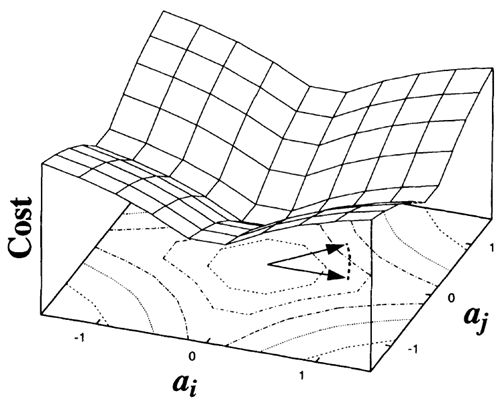
FIG. 2 The cost function for sparseness, plotted as a function of the joint activity of two coefficients, \(a_i\) and \(a_j\). In this example, \(S(x) = \log(1 + x^2)\). An activity vector that points towards a corner, where activity is distributed equally between coefficients, will incur a higher cost than a vector with the
same length that lies along one of the axes, where the total activity is loaded onto one coefficient. The gradient tends to ‘sparsify’ activity by differentially reducing the value of low-activity coefficients more than high-activity coefficients. Alternatively, the sparseness cost function may be interpreted as the negative logarithm of the prior probability of the \(a_i\) (ref. 23), assuming
statistical independence among the \(a_i\) (that is, a factorial distribution), and with the shape of the distribution specified by \(S\) (in this case a Cauchy distribution).(4.0 bits compared with 4.6 bits before training), and increased
kurtosis (20 compared with 7.0) for a mean-square reconstruction
error that is 10% of the image variance.
図2 スパースネスのコスト関数。2つの係数\(a_i\)と\(a_j\)の結合アクティビティの関数としてプロットされている。この例では、\(S(x) = \log(1 + x^2)\)である。アクティビティベクトルが角を指し、アクティビティが係数間で均等に分散されている場合、同じ長さのベクトルがいずれかの軸に沿って位置し、合計アクティビティが1つの係数に集中している場合よりもコストが高くなる。勾配は、低アクティビティ係数の値を高アクティビティ係数よりも差別的に減少させることで、アクティビティを「スパース化」する傾向がある。あるいは、スパース性コスト関数は、\(a_i\) の事前確率の負の対数として解釈することもできる (文献 23)。この場合、\(a_i\) 間の統計的独立性(つまり、因子分布)と、\(S\) によって指定される分布の形状(この場合はコーシー分布)を仮定する。(トレーニング前の 4.6 ビットに対して 4.0 ビット)、および画像分散の 10% の平均二乗再構成誤差に対する尖度の増加(7.0 に対して 20)が想定される。
Learning is accomplished by minimizing the total cost func-
tional, \(E\) (equation (2)). For each image presentation, \(E\) is
minimized with respect to the \(a_i\). The \(\phi_i\) then evolve by gradient
descent on \(E\) averaged over many image presentations. Thus for a
given image, the \(a_i\) are determined from the equilibrium solution
to the differential equation:
学習は、総コスト関数 \(E\)(式(2))を最小化することによって達成される。各画像提示において、\(E\)は\(a_i\)に関して最小化される。そして、\(\phi_i\)は、多数の画像提示にわたって平均化された\(E\)に基づく勾配降下法によって進化する。したがって、与えられた画像について、\(a_i\)は微分方程式の平衡解から決定される。
\[
\dot{a}_i = b_i - \sum_j C_{ij}a_j - \frac{λ}{σ}S^\prime\left(\frac{a_i}{σ}\right) \tag{5}
\]
where \(b_i=\sum_{x,y}\phi_i(x,y)I(x,y)\) and \(C_{ij}=\sum_{x,y}\phi_i(x,y)\phi_j(x,y)\). The learning rule for updating the \(\phi\) is then:
ここで、\(b_i=\sum_{x,y}\phi_i(x,y)I(x,y)\) かつ \(C_{ij}=\sum_{x,y}\phi_i(x,y)\phi_j(x,y)\) である。\(\phi\) を更新するための学習則は以下の通りである。
\[
Δ\phi_i(x_m,y_n)=η\langle a_i\left[I(x_m,y_n)-\hat{I}(x_m,y_n)\right]\rangle \tag{6}
\]
where \(\hat{I}\) is the reconstructed image, \(\hat{I}(x_m,y_n) = \sum_i a_i\phi_i(x_m,y_n)\), and \(η\) is the learning rate. One can see from inspection of equations (5)
and (6) that the dynamics of the \(a_i\), as well as the learning rule for
the \(\phi_i\), have a local network implementation. An intuitive way of
understanding the algorithm is that it is seeking a set of \(\phi_i\) for
which the \(a_i\) can tolerate ‘sparsification’ with minimum reconstruc-
tion error. Importantly, the algorithm allows for the basis func-
tions to be overcomplete (that is, more basis functions than
meaningful dimensions in the input) and non-orthogonal5, with-
out reducing the degree of sparseness in the representation. This
is because the sparseness cost function, \(S\), forces the system to
choose, in the case of overlaps, which basis functions are most
effective for describing a given structure in the image.
ここで、\(\hat{I}\) は再構成画像、\(\hat{I}(x_m,y_n) = \sum_i a_i\phi_i(x_m,y_n)\)、
\(η\) は学習率です。式 (5)
と (6) を調べると、\(a_i\) のダイナミクスと、\(\phi_i\) の学習則は、ローカルネットワーク実装されていることがわかります。このアルゴリズムを直感的に理解するには、\(a_i\) が再構成誤差を最小に抑えながら「スパース化」を許容できる \(\phi_i\) の集合を求めていると考えます。重要なのは、このアルゴリズムでは、表現のスパース性を損なうことなく、基底関数が過剰完備(つまり、入力の有効な次元よりも多くの基底関数)かつ非直交5であっても構わないという点です。これは、スパース性コスト関数\(S\)により、重なりがある場合に、画像内の特定の構造を記述するのに最も効果的な基底関数をシステムが選択する必要があるためです。
The learning rule (equation (6)) was tested on several artificial
datasets containing controlled forms of sparse structure, and the
results of these tests (Fig. 3) confirm that the algorithm is indeed
capable of discovering sparse structure in input data, even when
the sparse components are non-orthogonal. The result of training
the system on 16 x 16 image patches extracted from natural
scenes is shown in Fig. 4a. The vast majority of basis functions
are well localized within each array (with the exception of the low-
frequency functions). Moreover, the functions are oriented and
selective to different spatial scales. This result should not come as
a surprise, because it simply reflects the fact that natural images
contain localized, oriented structures with limited phase align-
ment across spatial frequency6. The functions \(\phi_i\) shown are the
feedforward weights that, in addition to other terms, contribute to
the value of each \(a_i\) (refer to term 5; in equation (5)). To establish
the correspondence to physiologically measured receptive fields,
we mapped out the response of each \(a_i\) to spots at every position:
the results of this analysis show that the receptive fields are very
similar in form to the basis functions (Fig. 4b). The entire set of
basis functions forms a complete image code that spans the joint
space of spatial position, orientation and scale (Fig. 4c) in a
manner similar to wavelet codes, which have previously been
shown to form sparse representations of natural images8,12,22.
The average spatial-frequency bandwidth is 1.1 octaves (s.d.,
0.5) with an average aspect ratio (length/width) of 1.3 (s.d., 0.5),
which are characteristics reasonably similar to those of simple-cell
receptive fields (~1.5 octaves, length/width ~2)5. The resulting
histograms have sparse distributions (Fig. 4d), decreased entropy
学習則(式(6))は、制御された形態のスパース構造を含むいくつかの人工データセットでテストされ、これらのテスト結果(図3)は、スパース成分が非直交の場合でも、アルゴリズムが入力データ内のスパース構造を実際に検出できることを確認したものです。自然風景から抽出された16×16の画像パッチでシステムを学習させた結果を図4aに示します。基底関数の大部分は、各配列内でよく局在しています(低周波関数を除く)。さらに、関数は異なる空間スケールに対して方向性があり、選択的です。この結果は驚くべきことではありません。なぜなら、これは自然画像が、空間周波数にわたって位相の整列が限られた、局所的で方向性のある構造を含むという事実を反映しているに過ぎないからです6。示されている関数\(\phi_i\)は、他の項に加えて、各\(a_i\)の値に寄与するフィードフォワード重みです(式(5)の項5を参照)。生理学的に測定された受容野との対応を確立するために、各\(a_i\)のあらゆる位置におけるスポットへの応答をマッピングしました。
この解析の結果、受容野は基底関数と非常に類似した形状をしていることがわかりました(図4b)。基底関数の全体セットは、空間位置、方向、スケールの結合空間に広がる完全な画像コードを形成します(図4c)。これは、ウェーブレットコードに類似しており、ウェーブレットコードは、以前に自然画像のスパース表現を形成することが示されています8,12,22。
平均空間周波数帯域幅は1.1オクターブ(標準偏差0.5)、平均アスペクト比(長さ/幅)は1.3(標準偏差0.5)であり、
これは単純細胞受容野(約1.5オクターブ、長さ/幅約2)5の特性とほぼ類似している。得られたヒストグラムは疎な分布を示し(図4d)、エントロピーは減少している。
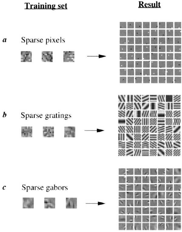
FIG. 3 Test cases. Representative training images are shown at the left and
the resulting basis functions that were learned from these examples are
shown at the right. In a, images were composed of sparse pixels: each pixel
was activated independently according to an exponential distribution,
\(P(x) =e^{-|x|}/Z\). In b, images were composed similarly to a, except with
gratings instead of pixels (that is, ‘sparse pixels’ in the Fourier domain). Inc,
images were composed of sparse, non-orthogonal Gabor functions with the
method described by Field12. In all cases, the basis functions were initialized
to random initial conditions. The learned basis functions successfully
recover the sparse components from which the images were, composed.
The form of the sparseness cost function was \(S(x) = -e^{-x^2}\), but other
choices (see text) yield the same results.
図3 テストケース。代表的なトレーニング画像を左側に示し、これらの例から学習された基底関数を右側に示します。aでは、画像はスパースピクセルで構成され、各ピクセルは指数分布\(P(x) = e^{-|x|}/Z\)に従って独立に活性化されました。bでは、画像はaと同様に構成されていますが、ピクセルの代わりに格子(つまり、フーリエ領域における「スパースピクセル」)が使用されています。bでは、画像はField12によって記述された方法を用いて、スパースで非直交なガボール関数で構成されています。すべてのケースにおいて、基底関数はランダムな初期条件に初期化されました。学習された基底関数は、画像を構成するスパース成分を正常に復元します。スパース性コスト関数の形式は\(S(x) = -e^{-x^2}\)ですが、他の選択肢(本文参照)でも同じ結果が得られます。
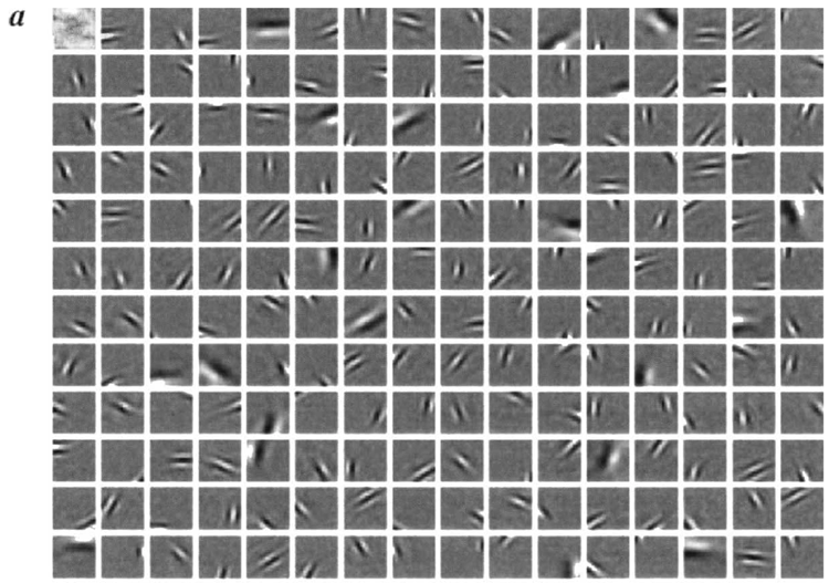

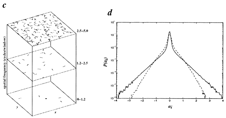
FIG. 4 Results from training a system of 192 basis functions
on 16 x 16-pixel image patches extracted form natural
scenes. The scenes were ten 512 x 512 images of natural
surroundings in the American northwest, preprocessed by
filtering with ia zero-phase_whitening/lowpass _ filter
\(R(f) = fe^{-(f/f_0)^4}, f_0 = 200\) cycles/picture (see also ref. 9).
Whitening na the fact that the mean-square error
(or m.s.e.) preferentially weights low frequencies for natural
scenes, whereas the attenuation at high spatial-frequencies
eliminates artefacts of rectangular sampling. The a, were
computed by the conjugate gradient method, halting when
the change in E was less than 1%. The \(\phi_i\) were initialized to
random values and were updated every 100 image presen-
tations. The vector length (gain) of each basis function, \(\phi_i\),
was adapted over time so as to maintain equal variance on
each coefficient. A stable solution was arrived at after
~4,000 updates (~400,000 image presentations). The
parameter \(λ\) was set so that \(λ/σ = 0.14\), with \(σ^2\) set to the
variance of the images. The form of the sparseness cost
function was \(S(x) = \log(1 + x^2)\). a, The learned basis func-
tions, scaled in magnitude so that each function fills the grey
scale, but with zero always represented by the same grey
level (black is negative, white is positive). b, The receptive
fields corresponding to the last row of basis functions in a,
obtained by mapping with spots (single pixels preprocessed
identically with the images). The principal difference may be
accounted for by the fact that sparsifying of activity makes
units more selective in which aspects of the stimulus they
respond to. c, The distribution of the learned basis functions
in space, orientation and scale. The functions were subdi-
vided into high-, medium- and low-spatial-frequency bands
(in octaves), according to the peak frequency in their power
spectra, and their spatial location was plotted within the
corresponding plane. Orientation preference is denoted by
line orientation. d, Activity histograms averaged over all
coefficients for the learned basis functions (solid line) and
for random initial conditions (broken line). In both cases,
\(λ/σ = 0.14\), showing that the learned basis functions can
accommodate a higher degree of sparsification. Note that
even the random basis functions have positive kurtosis due
to sparsification. The width of each bin used in calculating the
entropy was 0.04.
図4 自然風景から抽出した16×16ピクセルの画像パッチを用いて、192個の基底関数からなるシステムを学習させた結果。シーンは、アメリカ北西部の自然環境を写した512×512の画像10枚で、前処理として、ゼロ位相白色化/ローパスフィルタ(\(R(f) = fe^{-(f/f_0)^4}, f_0 = 200\)サイクル/画像)によるフィルタリングが施されている(文献9も参照)。白色化は、平均二乗誤差(m.s.e.)が自然風景の低周波数帯域に重点を置くのに対し、高空間周波数帯域での減衰によって矩形サンプリングのアーティファクトが除去されるという事実に基づいている。aは共役勾配法によって計算され、Eの変化が1%未満になった時点で停止した。 \(\phi_i\) はランダムな値に初期化され、100 枚の画像提示ごとに更新されました。各基底関数のベクトル長(ゲイン)\(\phi_i\) は、各係数の分散が等しくなるように時間の経過とともに適応されました。安定した解は、約 4,000 回の更新(約 400,000 枚の画像提示)後に得られました。パラメータ \(λ\) は \(λ/σ = 0.14\) となるように設定され、\(σ^2\) は画像の分散に設定されました。スパース性コスト関数の形式は \(S(x) = \log(1 + x^2)\) でした。a、学習された基底関数。各関数がグレースケールを埋めるように大きさが調整されていますが、ゼロは常に同じグレーレベル(黒は負、白は正)で表されます。 b, aの基底関数の最終行に対応する受容野。スポット(画像と同様に前処理された単一ピクセル)によるマッピングによって得られた。主な違いは、活動のスパース化によって、ユニットが刺激のどの側面に反応するかについて、より選択的になるという事実によって説明できる。c, 学習した基底関数の分布。関数は、パワースペクトルのピーク周波数に応じて、高、中、低空間周波数帯域(オクターブ単位)に分割され、対応する平面内に空間位置がプロットされた。方向の好みは線の向きで示されている。d, 学習した基底関数(実線)とランダム初期条件(破線)のすべての係数について平均した活動ヒストグラム。どちらの場合も、λ/σ = 0.14であり、学習した基底関数はより高度なスパース化に対応できることがわかる。ランダム基底関数であっても、スパース化により
正の尖度を持つことに留意してください。エントロピーの計算に使用した各ビンの幅は
0.04でした。
These results demonstrate that localized, oriented, bandpass
receptive fields emerge when only two global objectives are placed
on a linear coding of natural images: that information be pre-
served, and that the representation be sparse. These two objec-
tives alone are sufficient to account for the principal spatial
properties of simple-cell receptive fields. A number of unsuper-
vised learning algorithms based on similar principles have been
proposed for finding efficient representations of data”*™, all of
which seem to have the potential to arrive at results like these.
What remains as a challenge for these algorithms, and also for
ours, is to provide an account of other response properties of
simple cells (for example, direction selectivity), as well as the
complex response properties of neurons at later stages of the
visual pathway, which are noted for being highly nonlinear. An
important question, then, is whether these higher-order proper-
ties can be understood by considering the remaining forms of
statistical dependence that exist in natural images.
これらの結果は、自然画像の線形符号化において、情報の保存と表現のスパース性という2つの全体的な目的のみを課すと、局所的で方向性のある帯域通過受容野が形成されることを示しています。この2つの目的のみで、単純細胞受容野の主要な空間特性を説明するのに十分です。データの効率的な表現を見つけるための、同様の原理に基づく教師なし学習アルゴリズムが数多く提案されており、いずれも今回のような結果に到達する可能性を秘めているように思われます。これらのアルゴリズム、そして我々のアルゴリズムにとって残された課題は、単純細胞の他の応答特性(例えば、方向選択性)だけでなく、視覚経路の後期段階にあるニューロンの複雑な応答特性(高度に非線形であることが知られています)を説明することです。したがって、重要な問題は、これらの高次特性が、自然画像に存在する残りの統計的依存性を考慮することで理解できるかどうかということです。
Received 10 November 1995; accepted 25 April 1996.
ACKNOWLEDGEMENTS. We thank M. Lewicki for helpful discussions at the inception of this work, and
C. Lee, C. Brody, G. Harpur, F. Girosi and M. Riesenhuber for useful input. This work was supported by
grants from NIMH to both authors. Part of this work was carried out at the Center for Biological and
Computational Learning at the Massachusetts Institute of Technology.
謝辞: 本研究の開始に際して有益な議論をしてくださったM. Lewicki氏、そして有益な情報をくださったC. Lee氏、C. Brody氏、G. Harpur氏、F. Girosi氏、M. Riesenhuber氏に感謝申し上げます。本研究は、両著者がNIMHから助成金を受けて実施されました。本研究の一部は、マサチューセッツ工科大学の生物学・計算学習センターで実施されました。